32 Evaluation of three linear regression models
- Dataset:
iris.csv - Algorithms:
- Simple Linear Regression
- Multiple Regression
- Neural Networks
32.1 Introduction
https://www.matthewrenze.com/workshops/practical-machine-learning-with-r/lab-3a-regression.html
32.2 Explore the Data
- Load Iris data
- Plot scatterplot
- Plot correlogram
data(iris)Create scatterplot matrix
plot(iris[1:4])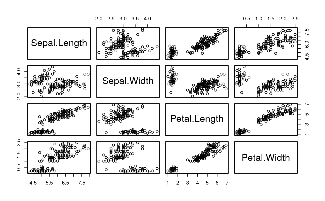
library(corrgram)
#> Registered S3 method overwritten by 'seriation':
#>   method         from
#>   reorder.hclust gclus
corrgram(iris[1:4])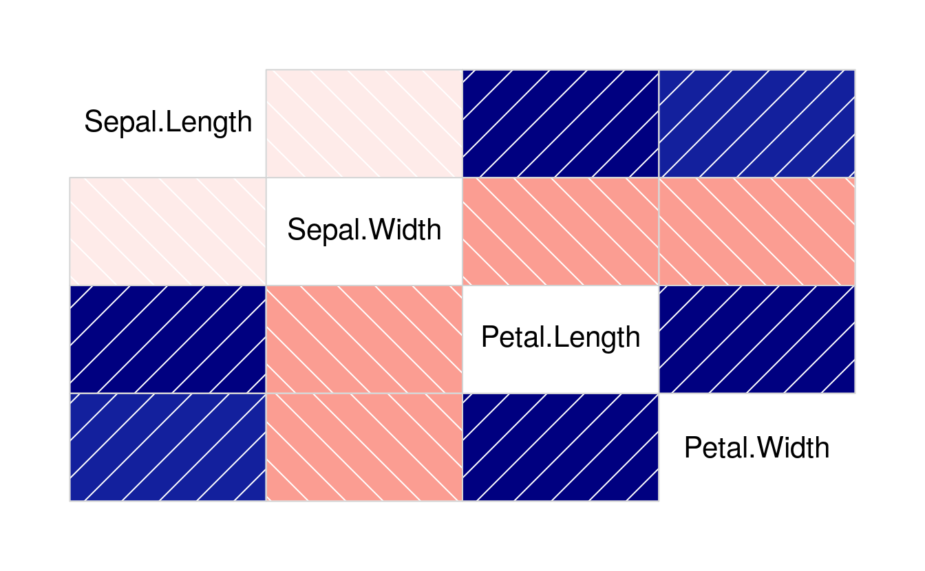
cor(iris[1:4])
#>              Sepal.Length Sepal.Width Petal.Length Petal.Width
#> Sepal.Length        1.000      -0.118        0.872       0.818
#> Sepal.Width        -0.118       1.000       -0.428      -0.366
#> Petal.Length        0.872      -0.428        1.000       0.963
#> Petal.Width         0.818      -0.366        0.963       1.000
cor(
  x = iris$Petal.Length,
  y = iris$Petal.Width)
#> [1] 0.963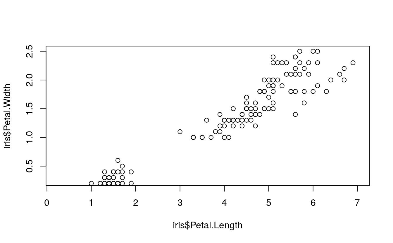
32.3 Create Training and Test Sets
set.seed(42)
indexes <- sample(
x = 1:150,
size = 100)
train <- iris[indexes, ]
test <- iris[-indexes, ]32.4 Predict with Simple Linear Regression
simpleModel <- lm(
formula = Petal.Width ~ Petal.Length,
data = train)
plot(
  x = iris$Petal.Length,
  y = iris$Petal.Width,
  xlim = c(0.25, 7),
  ylim = c(0.25, 2.5))
lines(
x = train$Petal.Length,
y = simpleModel$fitted,
col = "red",
lwd = 3)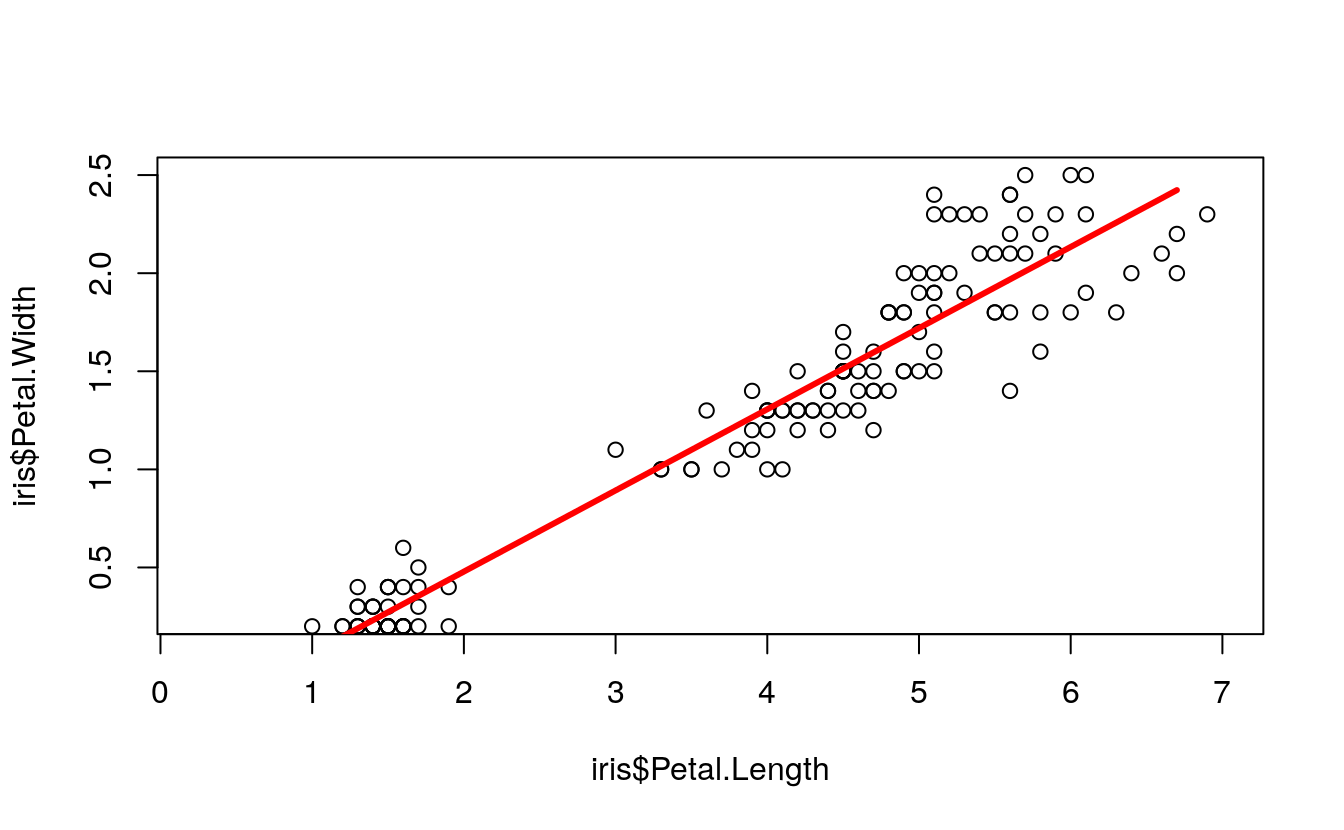
summary(simpleModel)
#>
#> Call:
#> lm(formula = Petal.Width ~ Petal.Length, data = train)
#>
#> Residuals:
#>     Min      1Q  Median      3Q     Max
#> -0.5684 -0.1279 -0.0307  0.1280  0.6385
#>
#> Coefficients:
#>              Estimate Std. Error t value Pr(>|t|)
#> (Intercept)   -0.3486     0.0476   -7.33  6.7e-11 ***
#> Petal.Length   0.4137     0.0119   34.80  < 2e-16 ***
#> ---
#> Signif. codes:  0 '***' 0.001 '**' 0.01 '*' 0.05 '.' 0.1 ' ' 1
#>
#> Residual standard error: 0.209 on 98 degrees of freedom
#> Multiple R-squared:  0.925,  Adjusted R-squared:  0.924
#> F-statistic: 1.21e+03 on 1 and 98 DF,  p-value: <2e-16
simplePredictions <- predict(
  object = simpleModel,
  newdata = test)
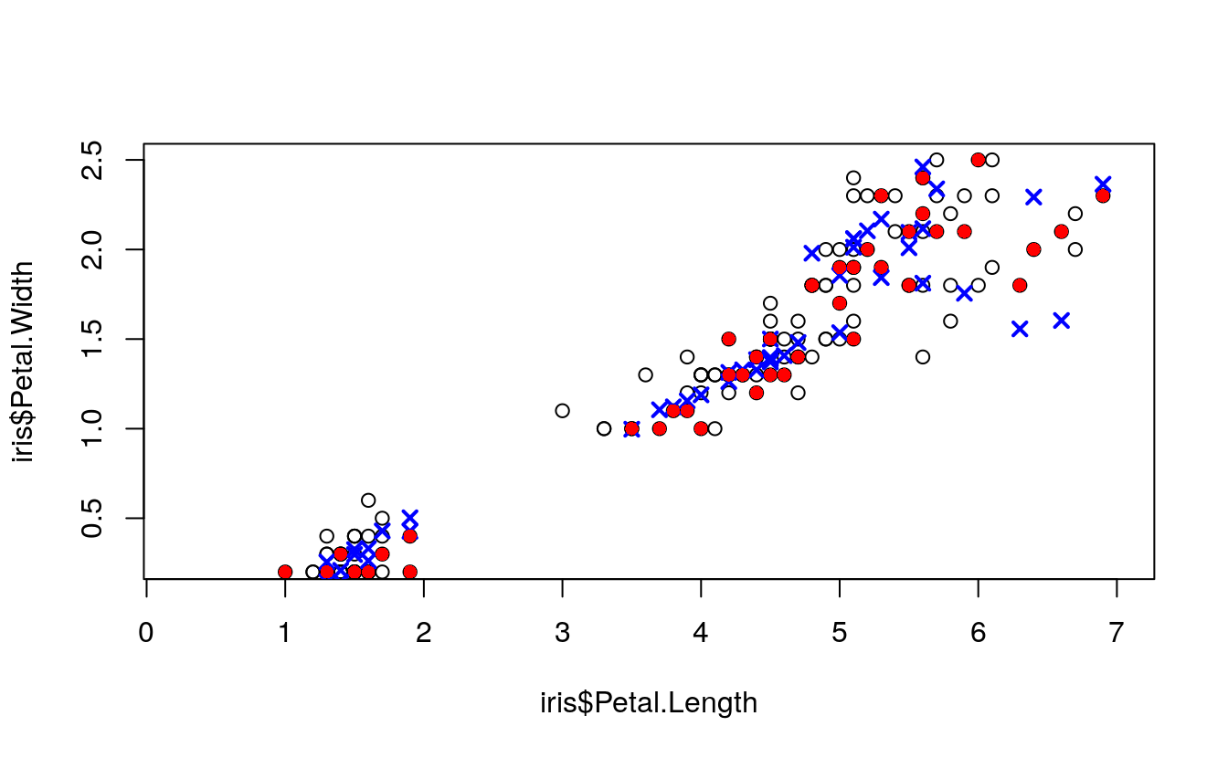
plot(
  x = iris$Petal.Length,
  y = iris$Petal.Width,
  xlim = c(0.25, 7),
  ylim = c(0.25, 2.5))

points(
  x = test$Petal.Length,
  y = simplePredictions,
  col = "blue",
  pch = 4,
  lwd = 2)

points(
  x = test$Petal.Length,
  y = test$Petal.Width,
  col = "red",
  pch = 16)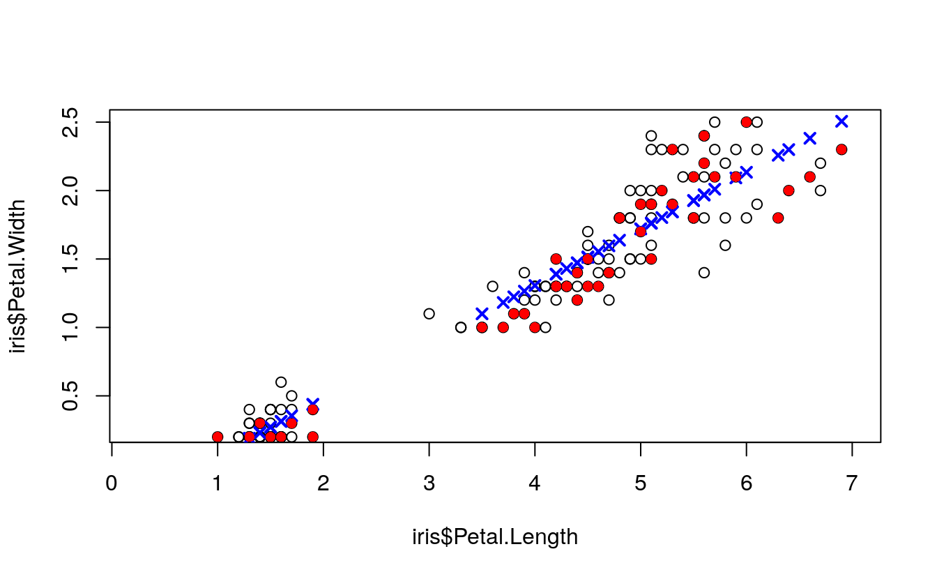
32.5 Predict with Multiple Regression
multipleModel <- lm(
  formula = Petal.Width ~ .,
  data = train)
summary(multipleModel)
#>
#> Call:
#> lm(formula = Petal.Width ~ ., data = train)
#>
#> Residuals:
#>     Min      1Q  Median      3Q     Max
#> -0.5769 -0.0843 -0.0066  0.0978  0.4731
#>
#> Coefficients:
#>                   Estimate Std. Error t value Pr(>|t|)
#> (Intercept)        -0.5088     0.2277   -2.23  0.02779 *
#> Sepal.Length       -0.0486     0.0593   -0.82  0.41435
#> Sepal.Width         0.2032     0.0594    3.42  0.00092 ***
#> Petal.Length        0.2103     0.0641    3.28  0.00146 **
#> Speciesversicolor   0.6769     0.1583    4.28  4.5e-05 ***
#> Speciesvirginica    1.0762     0.2126    5.06  2.1e-06 ***
#> ---
#> Signif. codes:  0 '***' 0.001 '**' 0.01 '*' 0.05 '.' 0.1 ' ' 1
#>
#> Residual standard error: 0.176 on 94 degrees of freedom
#> Multiple R-squared:  0.949,  Adjusted R-squared:  0.947
#> F-statistic:  352 on 5 and 94 DF,  p-value: <2e-16
multiplePredictions <- predict(
  object = multipleModel,
  newdata = test)
plot(
  x = iris$Petal.Length,
  y = iris$Petal.Width,
  xlim = c(0.25, 7),
  ylim = c(0.25, 2.5))

points(
  x = test$Petal.Length,
  y = multiplePredictions,
  col = "blue",
  pch = 4,
  lwd = 2)

points(
  x = test$Petal.Length,
  y = test$Petal.Width,
  col = "red",
  pch = 16)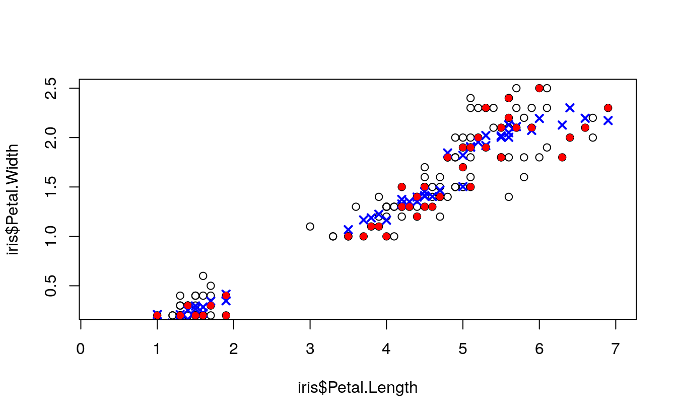
32.6 5. Predict with Neural Network Regression
scaledIris <- data.frame(
  Sepal.Length = normalize(iris$Sepal.Length),
  Sepal.Width = normalize(iris$Sepal.Width),
  Petal.Length = normalize(iris$Petal.Length),
  Petal.Width = normalize(iris$Petal.Width),
  Species = iris$Species)
scaledTrain <- scaledIris[indexes, ]
scaledTest <- scaledIris[-indexes, ]
library(nnet)

neuralRegressor <- nnet(
  formula = Petal.Width ~ .,
  data = scaledTrain,
  linout = TRUE,
  skip = TRUE,
  size = 4,
  decay = 0.0001,
  maxit = 500)
#> # weights:  34
#> initial  value 64.175158
#> iter  10 value 0.498340
#> iter  20 value 0.439307
#> iter  30 value 0.419373
#> iter  40 value 0.415119
#> iter  50 value 0.412305
#> iter  60 value 0.410862
#> iter  70 value 0.404854
#> iter  80 value 0.402606
#> iter  90 value 0.397903
#> iter 100 value 0.396295
#> iter 110 value 0.394292
#> iter 120 value 0.392628
#> iter 130 value 0.390306
#> iter 140 value 0.389577
#> iter 150 value 0.388916
#> iter 160 value 0.387607
#> iter 170 value 0.382857
#> iter 180 value 0.377332
#> iter 190 value 0.371974
#> iter 200 value 0.366019
#> iter 210 value 0.357405
#> iter 220 value 0.351831
#> iter 230 value 0.347613
#> iter 240 value 0.344466
#> iter 250 value 0.341515
#> iter 260 value 0.340828
#> iter 270 value 0.340236
#> iter 280 value 0.338736
#> iter 290 value 0.337991
#> iter 300 value 0.336182
#> iter 310 value 0.333793
#> iter 320 value 0.331206
#> iter 330 value 0.330171
#> iter 340 value 0.329803
#> iter 350 value 0.329587
#> iter 360 value 0.329343
#> iter 370 value 0.328909
#> iter 380 value 0.327579
#> iter 390 value 0.326227
#> iter 400 value 0.323911
#> iter 410 value 0.322154
#> iter 420 value 0.320878
#> iter 430 value 0.320122
#> iter 440 value 0.319153
#> iter 450 value 0.318239
#> iter 460 value 0.316869
#> iter 470 value 0.315668
#> iter 480 value 0.314685
#> iter 490 value 0.314604
#> iter 500 value 0.314257
#> final  value 0.314257
#> stopped after 500 iterations
scaledPredictions <- predict(
  object = neuralRegressor,
  newdata = scaledTest)
neuralPredictions <- denormalize(
  x = scaledPredictions,
  y = iris$Petal.Width)
plot(
  x = iris$Petal.Length,
  y = iris$Petal.Width,
  xlim = c(0.25, 7),
  ylim = c(0.25, 2.5))

points(
  x = test$Petal.Length,
  y = neuralPredictions,
  col = "blue",
  pch = 4,
  lwd = 2)

points(
  x = test$Petal.Length,
  y = test$Petal.Width,
  col = "red",
  pch = 16)