28 Predicting Flu outcome comparing eight classification algorithms
- Datasets:
fluH7N9_china_2013 - Algorithms: RF, GLMNET, KNN, PDA, LDA, NSC, C5, PLS
28.1 Introduction
Among the many nice R packages containing data collections is the outbreaks package. It contains datsets on epidemics and among them is data from the 2013 outbreak of influenza A H7N9 in China as analysed by Kucharski et al. (2014):
A. Kucharski, H. Mills, A. Pinsent, C. Fraser, M. Van Kerkhove, C. A. Donnelly, and S. Riley. 2014. Distinguishing between reservoir exposure and human-to-human transmission for emerging pathogens using case onset data. PLOS Currents Outbreaks. Mar 7, edition 1. doi: 10.1371/currents.outbreaks.e1473d9bfc99d080ca242139a06c455f.
A. Kucharski, H. Mills, A. Pinsent, C. Fraser, M. Van Kerkhove, C. A. Donnelly, and S. Riley. 2014. Data from: Distinguishing between reservoir exposure and human-to-human transmission for emerging pathogens using case onset data. Dryad Digital Repository. http://dx.doi.org/10.5061/dryad.2g43n.
28.1.1 Algorithms
We compare these classification algorithms:
- Random Forest
- GLM net
- k-Nearest Neighbors
- Penalized Discriminant Analysis
- Stabilized Linear Discriminant Analysis
- Nearest Shrunken Centroids
- Single C5.0 Tree
- Partial Least Squares
28.1.2 Workflow
- Load dataset
- Data wrangling
- Many dates as one variable:
gather - Convert group to factor:
factor - Change dates descriptions:
dplyr::mapvalues - Set several provinces as Other:
mapvalues - Convert gender to factor
- Convert province to factor
- Features visualization
- Area density plot of Month vs Age by Province, by date group, by outcome, by gender
- Number of flu cases by gender, by province
- Age density plot of flu cases by outcome
- Days passed from outset by province, by age, by gender, by outcome
- Feature engineering
- Generate new features
- Gender to numeric
- Provinces to binary classifiers
- Outcome to binary classifier
- Impute missing data:
mice
- Split dataset in training, validation and test sets
- Feature importance
- with Decision Trees
- with Random Forest
- Wrangling dataset
- Plot Importance vs Variable
- Impact on Datasets
- Density plot of training, validation and test datasets
- Features vs outcome by age, days onset to hospital, day onset to outcome
- Train models on training validation dataset
-
Numeric and visual Comparison of models
- Accuracy
- Kappa
-
Compare predictions on training validation set
- Create dataset for results
- New variable for outcome
- Predicting on unknown outcomes on training data
-
Numeric and visual Comparison of models
- Accuracy
- Kappa
-
Compare predictions on training validation set
- Create dataset for results
- New variable for outcome
Calculate predicted outcome
Save to CSV file
Calculate recovery cases
Summarize outcome
Plot month vs log2-ratio of recovery vs death, by gender, by age, by date group
28.1.3 Can we predict flu outcome with Machine Learning in R?
I will be using their data as an example to show how to use Machine Learning algorithms for predicting disease outcome.
To do so, I selected and extracted features from the raw data, including age, days between onset and outcome, gender, whether the patients were hospitalized, etc. Missing values were imputed and different model algorithms were used to predict outcome (death or recovery). The prediction accuracy, sensitivity and specificity. The thus prepared dataset was divided into training and testing subsets. The test subset contained all cases with an unknown outcome. Before I applied the models to the test data, I further split the training data into validation subsets.
The tested modeling algorithms were similarly successful at predicting the outcomes of the validation data. To decide on final classifications, I compared predictions from all models and defined the outcome “Death” or “Recovery” as a function of all models, whereas classifications with a low prediction probability were flagged as “uncertain”. Accounting for this uncertainty led to a 100% correct classification of the validation test set.
The training cases with unknown outcome were then classified based on the same algorithms. From 57 unknown cases, 14 were classified as “Recovery”, 10 as “Death” and 33 as uncertain.
In a Part 2, I am looking at how extreme gradient boosting performs on this dataset.
Disclaimer: I am not an expert in Machine Learning. Everything I know, I taught myself during the last months. So, if you see any mistakes or have tips and tricks for improvement, please don’t hesitate to let me know! Thanks. :-)
28.2 The data
The dataset contains case ID, date of onset, date of hospitalization, date of outcome, gender, age, province and of course the outcome: Death or Recovery. I can already see that there are a couple of missing values in the data, which I will deal with later.
options(width = 1000)

if (!require("outbreaks")) install.packages("outbreaks")
#> Loading required package: outbreaks
library(outbreaks)

fluH7N9_china_2013_backup <- fluH7N9_china_2013

fluH7N9_china_2013$age[which(fluH7N9_china_2013$age == "?")] <- NA
fluH7N9_china_2013$case_ID <- paste("case",
                                    fluH7N9_china_2013$case_id,
                                    sep = "_")
head(fluH7N9_china_2013)
#>   case_id date_of_onset date_of_hospitalisation date_of_outcome outcome gender age province case_ID
#> 1       1    2013-02-19                    <NA>      2013-03-04   Death      m  87 Shanghai  case_1
#> 2       2    2013-02-27              2013-03-03      2013-03-10   Death      m  27 Shanghai  case_2
#> 3       3    2013-03-09              2013-03-19      2013-04-09   Death      f  35    Anhui  case_3
#> 4       4    2013-03-19              2013-03-27            <NA>    <NA>      f  45  Jiangsu  case_4
#> 5       5    2013-03-19              2013-03-30      2013-05-15 Recover      f  48  Jiangsu  case_5
#> 6       6    2013-03-21              2013-03-28      2013-04-26   Death      f  32  Jiangsu  case_6
Before I start preparing the data for Machine Learning, I want to get an idea of the distribution of the data points and their different variables by plotting.
Most provinces have only a handful of cases, so I am combining them into the category “other” and keep only Jiangsu, Shanghai and Zhejian and separate provinces.
# make tidy data, clean up and simplify
library(tidyr)

# put different type of dates in one variable (Date)
fluH7N9_china_2013_gather <- fluH7N9_china_2013 %>%
  gather(Group, Date, date_of_onset:date_of_outcome)

# convert Group to factor
fluH7N9_china_2013_gather$Group <- factor(fluH7N9_china_2013_gather$Group,
                                          levels = c("date_of_onset",
                                                     "date_of_hospitalisation",
                                                     "date_of_outcome"))

# change the dates description with plyr::mapvalues
library(plyr)
from <- c("date_of_onset", "date_of_hospitalisation", "date_of_outcome")
to <- c("Date of onset", "Date of hospitalisation", "Date of outcome")
fluH7N9_china_2013_gather$Group <- mapvalues(fluH7N9_china_2013_gather$Group,
                                             from = from, to = to)

# change additional provinces to Other
from <- c("Anhui", "Beijing", "Fujian", "Guangdong", "Hebei", "Henan",
          "Hunan", "Jiangxi", "Shandong", "Taiwan")
to <- rep("Other", 10)
fluH7N9_china_2013_gather$province <-
  mapvalues(fluH7N9_china_2013_gather$province,
            from = from, to = to)

# convert gender to factor
levels(fluH7N9_china_2013_gather$gender) <-
  c(levels(fluH7N9_china_2013_gather$gender), "unknown")

# replace NA in gender by "unknown
is_na <- is.na(fluH7N9_china_2013_gather$gender)
fluH7N9_china_2013_gather$gender[is_na] <- "unknown"

# convert province to factor
fluH7N9_china_2013_gather$province <- factor(fluH7N9_china_2013_gather$province,
                                             levels = c("Jiangsu",  "Shanghai",
                                                        "Zhejiang", "Other"))
library(ggplot2)
my_theme <- function(base_size = 12, base_family = "sans"){
  theme_minimal(base_size = base_size, base_family = base_family) +
  theme(
    axis.text = element_text(size = 12),
    axis.text.x = element_text(angle = 45, vjust = 0.5, hjust = 0.5),
    axis.title = element_text(size = 14),
    panel.grid.major = element_line(color = "grey"),
    panel.grid.minor = element_blank(),
    panel.background = element_rect(fill = "aliceblue"),
    strip.background = element_rect(fill = "lightgrey", color = "grey",
                                    size = 1),
    strip.text = element_text(face = "bold", size = 12, color = "black"),
    legend.position = "bottom",
    legend.justification = "top",
    legend.box = "horizontal",
    legend.box.background = element_rect(colour = "grey50"),
    legend.background = element_blank(),
    panel.border = element_rect(color = "grey", fill = NA, size = 0.5)
  )
}
ggplot(data = fluH7N9_china_2013_gather,
       aes(x = Date, y = as.numeric(age), fill = outcome)) +
  stat_density2d(aes(alpha = ..level..), geom = "polygon") +
  geom_jitter(aes(color = outcome, shape = gender), size = 1.5) +
  geom_rug(aes(color = outcome)) +
  labs(
    fill = "Outcome",
    color = "Outcome",
    alpha = "Level",
    shape = "Gender",
    x = "Date in 2013",
    y = "Age",
    title = "2013 Influenza A H7N9 cases in China",
    subtitle = "Dataset from 'outbreaks' package (Kucharski et al. 2014)",
    caption = ""
  ) +
  facet_grid(Group ~ province) +
  my_theme() +
  scale_shape_manual(values = c(15, 16, 17)) +
  scale_color_brewer(palette="Set1", na.value = "grey50") +
  scale_fill_brewer(palette="Set1")
#> Warning: Removed 149 rows containing non-finite values (stat_density2d).
#> Warning: Removed 149 rows containing missing values (geom_point).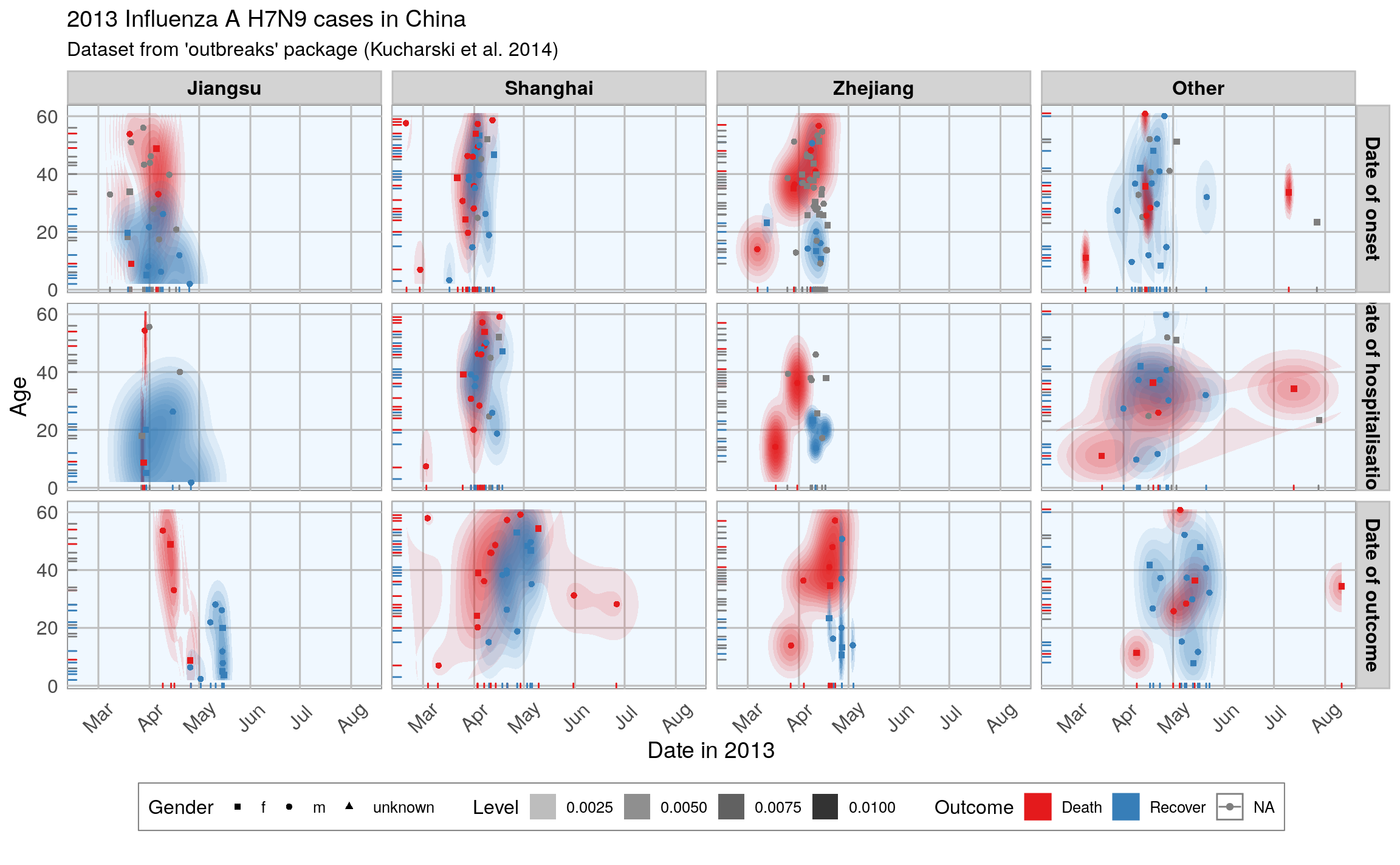
This plot shows the dates of onset, hospitalization and outcome (if known) of each data point. Outcome is marked by color and age shown on the y-axis. Gender is marked by point shape.
The density distribution of date by age for the cases seems to indicate that older people died more frequently in the Jiangsu and Zhejiang province than in Shanghai and in other provinces.
When we look at the distribution of points along the time axis, it suggests that their might be a positive correlation between the likelihood of death and an early onset or early outcome.
I also want to know how many cases there are for each gender and province and compare the genders’ age distribution.
# more tidy data. first remove age
fluH7N9_china_2013_gather_2 <- fluH7N9_china_2013_gather[, -4] %>%
  gather(group_2, value, gender:province)
#> Warning: attributes are not identical across measure variables;
#> they will be dropped

# change descriptions
from <- c("m", "f", "unknown", "Other")
to <- c("Male", "Female", "Unknown gender", "Other province")
fluH7N9_china_2013_gather_2$value <- mapvalues(fluH7N9_china_2013_gather_2$value,
                                               from = from, to = to)
# convert to factor
fluH7N9_china_2013_gather_2$value <- factor(fluH7N9_china_2013_gather_2$value,
                                            levels = c("Female", "Male",
                                                       "Unknown gender",
                                                       "Jiangsu", "Shanghai",
                                                       "Zhejiang", "Other
                                                       province"))

p1 <- ggplot(data = fluH7N9_china_2013_gather_2, aes(x = value,
                                                     fill = outcome,
                                                     color = outcome)) +
  geom_bar(position = "dodge", alpha = 0.7, size = 1) +
  my_theme() +
  scale_fill_brewer(palette="Set1", na.value = "grey50") +
  scale_color_brewer(palette="Set1", na.value = "grey50") +
  labs(
    color = "",
    fill = "",
    x = "",
    y = "Count",
    title = "2013 Influenza A H7N9 cases in China",
    subtitle = "Gender and Province numbers of flu cases",
    caption = ""
  )

p2 <- ggplot(data = fluH7N9_china_2013_gather, aes(x = as.numeric(age),
                                                   fill = outcome,
                                                   color = outcome)) +
  geom_density(alpha = 0.3, size = 1) +
  geom_rug() +
  scale_color_brewer(palette="Set1", na.value = "grey50") +
  scale_fill_brewer(palette="Set1", na.value = "grey50") +
  my_theme() +
  labs(
    color = "",
    fill = "",
    x = "Age",
    y = "Density",
    title = "",
    subtitle = "Age distribution of flu cases",
    caption = ""
  )

library(gridExtra)
library(grid)

grid.arrange(p1, p2, ncol = 2)
#> Warning: Removed 6 rows containing non-finite values (stat_density).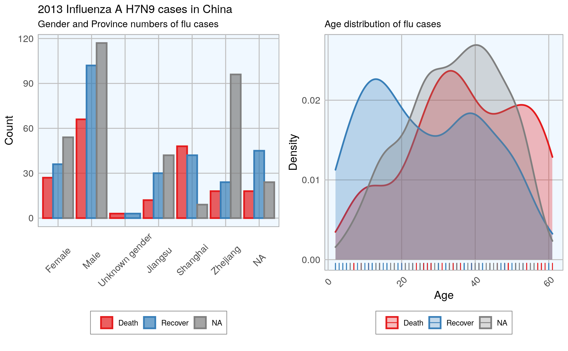
In the dataset, there are more male than female cases and correspondingly, we see more deaths, recoveries and unknown outcomes in men than in women. This is potentially a problem later on for modeling because the inherent likelihoods for outcome are not directly comparable between the sexes.
Most unknown outcomes were recorded in Zhejiang. Similarly to gender, we don’t have an equal distribution of data points across provinces either.
When we look at the age distribution it is obvious that people who died tended to be slightly older than those who recovered. The density curve of unknown outcomes is more similar to that of death than of recovery, suggesting that among these people there might have been more deaths than recoveries.
And lastly, I want to plot how many days passed between onset, hospitalization and outcome for each case.
ggplot(data = fluH7N9_china_2013_gather, aes(x = Date, y = as.numeric(age),
                                             color = outcome)) +
  geom_point(aes(color = outcome, shape = gender), size = 1.5, alpha = 0.6) +
  geom_path(aes(group = case_ID)) +
  facet_wrap( ~ province, ncol = 2) +
  my_theme() +
  scale_shape_manual(values = c(15, 16, 17)) +
  scale_color_brewer(palette="Set1", na.value = "grey50") +
  scale_fill_brewer(palette="Set1") +
  labs(
    color = "Outcome",
    shape = "Gender",
    x = "Date in 2013",
    y = "Age",
    title = "2013 Influenza A H7N9 cases in China",
    subtitle = "Dataset from 'outbreaks' package (Kucharski et al. 2014)",
    caption = "\nTime from onset of flu to outcome."
  )
#> Warning: Removed 149 rows containing missing values (geom_point).
#> Warning: Removed 122 row(s) containing missing values (geom_path).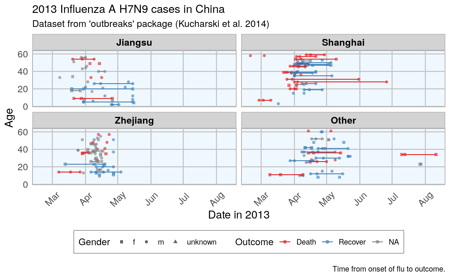
This plot shows that there are many missing values in the dates, so it is hard to draw a general conclusion.
28.3 Features
In Machine Learning-speak features are the variables used for model training. Using the right features dramatically influences the accuracy of the model. Because we don’t have many features, I am keeping age as it is, but I am also generating new features:
from the date information I am calculating the days between onset and outcome and between onset and hospitalization
I am converting gender into numeric values with 1 for female and 0 for male
similarly, I am converting provinces to binary classifiers (yes == 1, no == 0) for Shanghai, Zhejiang, Jiangsu and other provinces
the same binary classification is given for whether a case was hospitalised, and whether they had an early onset or early outcome (earlier than the median date)
# convert gender, provinces to discrete and numeric values
library(dplyr)
#>
#> Attaching package: 'dplyr'
#> The following object is masked from 'package:gridExtra':
#>
#>     combine
#> The following objects are masked from 'package:plyr':
#>
#>     arrange, count, desc, failwith, id, mutate, rename, summarise, summarize
#> The following objects are masked from 'package:stats':
#>
#>     filter, lag
#> The following objects are masked from 'package:base':
#>
#>     intersect, setdiff, setequal, union

dataset <- fluH7N9_china_2013 %>%
  mutate(hospital = as.factor(ifelse(is.na(date_of_hospitalisation), 0, 1)),
         gender_f = as.factor(ifelse(gender == "f", 1, 0)),
         province_Jiangsu = as.factor(ifelse(province == "Jiangsu", 1, 0)),
         province_Shanghai = as.factor(ifelse(province == "Shanghai", 1, 0)),
         province_Zhejiang = as.factor(ifelse(province == "Zhejiang", 1, 0)),
         province_other = as.factor(ifelse(province == "Zhejiang" |
                                             province == "Jiangsu" |
                                             province == "Shanghai", 0, 1)),
         days_onset_to_outcome = as.numeric(as.character(gsub(" days", "",
                as.Date(as.character(date_of_outcome), format = "%Y-%m-%d") -
                as.Date(as.character(date_of_onset), format = "%Y-%m-%d")))),

         days_onset_to_hospital = as.numeric(as.character(gsub(" days", "",
            as.Date(as.character(date_of_hospitalisation), format = "%Y-%m-%d") -
            as.Date(as.character(date_of_onset), format = "%Y-%m-%d")))),
         age = as.numeric(as.character(age)),
         early_onset = as.factor(ifelse(date_of_onset <
                        summary(date_of_onset)[[3]], 1, 0)),
         early_outcome = as.factor(ifelse(date_of_outcome <
                        summary(date_of_outcome)[[3]], 1, 0))) %>%
  subset(select = -c(2:4, 6, 8))
  # print

rownames(dataset) <- dataset$case_ID
dataset <- dataset[, -c(1,4)]
head(dataset)
#>        outcome age hospital gender_f province_Jiangsu province_Shanghai province_Zhejiang province_other days_onset_to_outcome days_onset_to_hospital early_onset early_outcome
#> case_1   Death  87        0        0                0                 1                 0              0                    13                     NA           1             1
#> case_2   Death  27        1        0                0                 1                 0              0                    11                      4           1             1
#> case_3   Death  35        1        1                0                 0                 0              1                    31                     10           1             1
#> case_4    <NA>  45        1        1                1                 0                 0              0                    NA                      8           1          <NA>
#> case_5 Recover  48        1        1                1                 0                 0              0                    57                     11           1             0
#> case_6   Death  32        1        1                1                 0                 0              0                    36                      7           1             1
summary(dataset$outcome)
#>   Death Recover    NA's
#>      32      47      57
28.3.1 Imputing missing values
https://www.r-bloggers.com/imputing-missing-data-with-r-mice-package/
When looking at the dataset I created for modeling, it is obvious that we have quite a few missing values.
The missing values from the outcome column are what I want to predict but for the rest I would either have to remove the entire row from the data or impute the missing information. I decided to try the latter with the mice package.
library(mice)
#>
#> Attaching package: 'mice'
#> The following objects are masked from 'package:base':
#>
#> cbind, rbind
dataset_impute <- mice(dataset[, -1], print = FALSE) # remove outcome
#> Warning: Number of logged events: 150
impute_complete <- mice::complete(dataset_impute, 1) # return 1st imputed dataset
rownames(impute_complete) <- row.names(dataset)
impute_complete
#> age hospital gender_f province_Jiangsu province_Shanghai province_Zhejiang province_other days_onset_to_outcome days_onset_to_hospital early_onset early_outcome
#> case_1 87 0 0 0 1 0 0 13 6 1 1
#> case_2 27 1 0 0 1 0 0 11 4 1 1
#> case_3 35 1 1 0 0 0 1 31 10 1 1
#> case_4 45 1 1 1 0 0 0 14 8 1 1
#> case_5 48 1 1 1 0 0 0 57 11 1 0
#> case_6 32 1 1 1 0 0 0 36 7 1 1
#> case_7 83 1 0 1 0 0 0 20 9 1 1
#> case_8 38 1 0 0 0 1 0 20 11 1 1
#> case_9 67 1 0 0 0 1 0 7 0 1 1
#> case_10 48 1 0 0 1 0 0 6 4 1 1
#> case_11 64 1 0 0 0 1 0 6 2 1 1
#> case_12 52 0 1 0 1 0 0 7 7 1 1
#> case_13 67 1 1 0 1 0 0 12 3 1 1
#> case_14 4 0 0 0 1 0 0 10 5 1 1
#> case_15 61 0 1 1 0 0 0 32 4 1 0
#> case_16 79 0 0 1 0 0 0 38 4 1 0
#> case_17 74 1 0 0 1 0 0 14 6 1 1
#> case_18 66 1 0 0 1 0 0 20 4 1 1
#> case_19 59 1 0 0 1 0 0 67 5 1 0
#> case_20 55 1 0 0 0 0 1 22 4 1 1
#> case_21 67 1 0 0 1 0 0 23 1 1 1
#> case_22 85 1 0 1 0 0 0 31 4 1 0
#> case_23 25 1 1 1 0 0 0 46 0 1 0
#> case_24 64 0 0 0 1 0 0 6 5 1 1
#> case_25 62 1 0 0 1 0 0 35 0 1 0
#> case_26 77 1 0 0 1 0 0 11 4 1 1
#> case_27 51 1 1 0 0 1 0 37 27 1 1
#> case_28 79 0 0 0 0 1 0 32 0 1 0
#> case_29 76 1 1 0 1 0 0 32 4 1 0
#> case_30 81 0 1 0 1 0 0 23 0 1 0
#> case_31 70 0 0 1 0 0 0 32 4 1 0
#> case_32 74 0 0 1 0 0 0 38 4 1 0
#> case_33 65 0 0 0 0 1 0 24 8 1 0
#> case_34 74 1 0 0 1 0 0 11 5 1 1
#> case_35 83 1 1 0 1 0 0 38 5 1 0
#> case_36 68 0 0 0 1 0 0 17 4 1 1
#> case_37 31 0 0 1 0 0 0 45 7 1 0
#> case_38 56 0 0 1 0 0 0 23 7 1 0
#> case_39 66 1 0 0 0 1 0 13 0 0 1
#> case_40 74 1 0 0 0 1 0 6 5 1 1
#> case_41 54 1 1 0 0 1 0 23 6 1 1
#> case_42 53 1 0 0 1 0 0 11 7 1 1
#> case_43 86 1 0 0 1 0 0 18 3 1 1
#> case_44 7 1 1 0 0 0 1 6 0 0 1
#> case_45 56 1 0 0 1 0 0 86 3 1 0
#> case_46 77 0 1 1 0 0 0 9 0 1 1
#> case_47 72 0 0 1 0 0 0 32 5 1 0
#> case_48 65 1 0 0 0 1 0 20 6 1 1
#> case_49 38 1 0 0 0 1 0 28 5 1 0
#> case_50 34 1 0 0 0 0 1 17 3 1 0
#> case_51 65 1 0 0 0 0 1 15 2 0 1
#> case_52 64 0 1 0 0 1 0 17 7 1 1
#> case_53 62 0 1 0 0 1 0 22 7 1 1
#> case_54 75 0 0 0 0 1 0 37 7 1 0
#> case_55 79 0 0 0 0 1 0 18 7 0 0
#> case_56 73 1 0 0 1 0 0 11 6 1 1
#> case_57 54 1 0 0 1 0 0 13 4 0 1
#> case_58 78 1 0 0 1 0 0 31 4 1 0
#> case_59 50 0 0 1 0 0 0 37 7 1 0
#> case_60 26 0 0 1 0 0 0 18 4 0 1
#> case_61 60 0 0 1 0 0 0 10 4 1 1
#> case_62 68 0 1 0 0 1 0 11 5 1 1
#> case_63 60 0 0 0 0 0 1 26 3 0 0
#> case_64 56 0 0 1 0 0 0 16 4 0 0
#> case_65 21 0 1 1 0 0 0 37 4 1 0
#> case_66 72 0 0 1 0 0 0 32 3 0 0
#> case_67 56 0 0 0 0 1 0 31 3 0 0
#> case_68 57 0 0 0 0 1 0 6 10 0 1
#> case_69 62 0 0 0 0 1 0 8 7 0 1
#> case_70 58 0 1 0 0 1 0 10 11 0 1
#> case_71 72 0 1 0 0 1 0 13 6 0 0
#> case_72 47 1 0 0 1 0 0 17 5 0 0
#> case_73 69 0 0 0 1 0 0 7 4 0 1
#> case_74 54 0 0 0 1 0 0 17 6 1 0
#> case_75 83 0 0 0 1 0 0 6 4 1 1
#> case_76 55 0 0 0 1 0 0 6 7 1 1
#> case_77 2 0 0 0 1 0 0 13 7 1 0
#> case_78 89 1 0 0 1 0 0 17 4 0 0
#> case_79 37 0 1 0 0 1 0 16 0 0 0
#> case_80 74 0 0 0 0 1 0 22 3 0 0
#> case_81 86 0 0 0 0 1 0 10 6 0 1
#> case_82 41 0 0 0 0 1 0 8 10 0 1
#> case_83 38 0 0 0 0 0 1 23 4 0 0
#> case_84 26 0 1 1 0 0 0 13 1 1 1
#> case_85 80 1 1 0 1 0 0 13 7 0 1
#> case_86 54 0 1 0 0 1 0 10 3 0 1
#> case_87 69 0 0 0 0 1 0 8 3 0 1
#> case_88 4 0 0 0 0 0 1 11 0 0 0
#> case_89 54 1 0 1 0 0 0 36 6 0 0
#> case_90 43 1 0 0 0 1 0 9 3 0 1
#> case_91 48 1 0 0 0 1 0 16 6 0 0
#> case_92 66 1 1 0 0 1 0 13 7 0 1
#> case_93 56 0 0 0 0 1 0 17 0 0 0
#> case_94 35 0 1 0 0 1 0 13 6 0 0
#> case_95 37 0 0 0 0 1 0 7 4 1 1
#> case_96 43 0 0 1 0 0 0 37 4 1 0
#> case_97 75 1 1 0 1 0 0 22 5 0 0
#> case_98 76 0 0 0 0 1 0 13 3 0 1
#> case_99 68 0 1 0 0 1 0 6 7 0 1
#> case_100 58 0 0 0 0 1 0 20 7 0 0
#> case_101 79 0 1 0 0 1 0 13 3 0 1
#> case_102 81 0 0 0 0 1 0 32 6 0 0
#> case_103 68 1 0 1 0 0 0 37 6 0 0
#> case_104 54 0 1 0 0 1 0 20 7 0 0
#> case_105 32 0 0 0 0 1 0 22 6 0 0
#> case_106 36 1 0 0 0 0 1 30 6 0 0
#> case_107 91 0 0 0 0 0 1 21 10 0 0
#> case_108 84 0 0 0 0 1 0 13 3 0 0
#> case_109 62 0 0 0 0 1 0 6 0 0 1
#> case_110 53 1 0 0 0 0 1 9 4 0 0
#> case_111 56 0 0 0 0 0 1 22 5 0 0
#> case_112 69 0 0 0 0 0 1 10 1 0 0
#> case_113 60 0 1 0 0 1 0 13 3 0 0
#> case_114 50 0 1 0 0 1 0 10 6 0 1
#> case_115 38 0 0 0 0 1 0 16 5 0 0
#> case_116 65 1 0 0 0 0 1 21 5 0 0
#> case_117 76 0 1 0 0 0 1 28 5 0 0
#> case_118 49 0 0 1 0 0 0 18 5 0 1
#> case_119 36 0 0 1 0 0 0 26 4 0 0
#> case_120 60 0 0 1 0 0 0 31 7 1 0
#> case_121 64 1 1 0 0 0 1 30 5 0 0
#> case_122 38 0 0 0 0 1 0 2 3 0 1
#> case_123 54 1 0 0 0 0 1 16 7 0 0
#> case_124 80 0 0 0 0 0 1 17 7 0 0
#> case_125 31 0 1 0 0 0 1 20 0 0 0
#> case_126 80 1 0 0 0 0 1 24 10 0 0
#> case_127 4 0 0 0 0 0 1 9 4 0 0
#> case_128 58 1 0 0 0 0 1 22 7 0 0
#> case_129 69 1 0 0 0 0 1 28 4 0 0
#> case_130 69 1 0 0 0 0 1 30 1 0 0
#> case_131 9 1 0 0 0 0 1 11 1 0 0
#> case_132 79 1 1 0 0 0 1 18 0 0 1
#> case_133 6 1 0 0 0 0 1 2 0 0 0
#> case_134 15 1 0 1 0 0 0 7 1 0 0
#> case_135 61 1 1 0 0 0 1 32 3 0 0
#> case_136 51 1 1 0 0 0 1 8 1 0 1
dataset_complete <- merge(dataset[, 1, drop = FALSE],
# mice::complete(dataset_impute, 1),
impute_complete,
by = "row.names", all = TRUE)
rownames(dataset_complete) <- dataset_complete$Row.names
dataset_complete <- dataset_complete[, -1]
dataset_complete
#> outcome age hospital gender_f province_Jiangsu province_Shanghai province_Zhejiang province_other days_onset_to_outcome days_onset_to_hospital early_onset early_outcome
#> case_1 Death 87 0 0 0 1 0 0 13 6 1 1
#> case_10 Death 48 1 0 0 1 0 0 6 4 1 1
#> case_100 <NA> 58 0 0 0 0 1 0 20 7 0 0
#> case_101 <NA> 79 0 1 0 0 1 0 13 3 0 1
#> case_102 <NA> 81 0 0 0 0 1 0 32 6 0 0
#> case_103 <NA> 68 1 0 1 0 0 0 37 6 0 0
#> case_104 <NA> 54 0 1 0 0 1 0 20 7 0 0
#> case_105 <NA> 32 0 0 0 0 1 0 22 6 0 0
#> case_106 Recover 36 1 0 0 0 0 1 30 6 0 0
#> case_107 Death 91 0 0 0 0 0 1 21 10 0 0
#> case_108 <NA> 84 0 0 0 0 1 0 13 3 0 0
#> case_109 <NA> 62 0 0 0 0 1 0 6 0 0 1
#> case_11 Death 64 1 0 0 0 1 0 6 2 1 1
#> case_110 <NA> 53 1 0 0 0 0 1 9 4 0 0
#> case_111 Death 56 0 0 0 0 0 1 22 5 0 0
#> case_112 <NA> 69 0 0 0 0 0 1 10 1 0 0
#> case_113 <NA> 60 0 1 0 0 1 0 13 3 0 0
#> case_114 <NA> 50 0 1 0 0 1 0 10 6 0 1
#> case_115 <NA> 38 0 0 0 0 1 0 16 5 0 0
#> case_116 Recover 65 1 0 0 0 0 1 21 5 0 0
#> case_117 Recover 76 0 1 0 0 0 1 28 5 0 0
#> case_118 <NA> 49 0 0 1 0 0 0 18 5 0 1
#> case_119 Recover 36 0 0 1 0 0 0 26 4 0 0
#> case_12 Death 52 0 1 0 1 0 0 7 7 1 1
#> case_120 <NA> 60 0 0 1 0 0 0 31 7 1 0
#> case_121 Death 64 1 1 0 0 0 1 30 5 0 0
#> case_122 <NA> 38 0 0 0 0 1 0 2 3 0 1
#> case_123 Death 54 1 0 0 0 0 1 16 7 0 0
#> case_124 Recover 80 0 0 0 0 0 1 17 7 0 0
#> case_125 Recover 31 0 1 0 0 0 1 20 0 0 0
#> case_126 <NA> 80 1 0 0 0 0 1 24 10 0 0
#> case_127 Recover 4 0 0 0 0 0 1 9 4 0 0
#> case_128 Recover 58 1 0 0 0 0 1 22 7 0 0
#> case_129 Recover 69 1 0 0 0 0 1 28 4 0 0
#> case_13 Death 67 1 1 0 1 0 0 12 3 1 1
#> case_130 <NA> 69 1 0 0 0 0 1 30 1 0 0
#> case_131 Recover 9 1 0 0 0 0 1 11 1 0 0
#> case_132 <NA> 79 1 1 0 0 0 1 18 0 0 1
#> case_133 Recover 6 1 0 0 0 0 1 2 0 0 0
#> case_134 Recover 15 1 0 1 0 0 0 7 1 0 0
#> case_135 Death 61 1 1 0 0 0 1 32 3 0 0
#> case_136 <NA> 51 1 1 0 0 0 1 8 1 0 1
#> case_14 Recover 4 0 0 0 1 0 0 10 5 1 1
#> case_15 <NA> 61 0 1 1 0 0 0 32 4 1 0
#> case_16 <NA> 79 0 0 1 0 0 0 38 4 1 0
#> case_17 Death 74 1 0 0 1 0 0 14 6 1 1
#> case_18 Recover 66 1 0 0 1 0 0 20 4 1 1
#> case_19 Death 59 1 0 0 1 0 0 67 5 1 0
#> case_2 Death 27 1 0 0 1 0 0 11 4 1 1
#> case_20 Recover 55 1 0 0 0 0 1 22 4 1 1
#> case_21 Recover 67 1 0 0 1 0 0 23 1 1 1
#> case_22 <NA> 85 1 0 1 0 0 0 31 4 1 0
#> case_23 Recover 25 1 1 1 0 0 0 46 0 1 0
#> case_24 Death 64 0 0 0 1 0 0 6 5 1 1
#> case_25 Recover 62 1 0 0 1 0 0 35 0 1 0
#> case_26 Death 77 1 0 0 1 0 0 11 4 1 1
#> case_27 Recover 51 1 1 0 0 1 0 37 27 1 1
#> case_28 <NA> 79 0 0 0 0 1 0 32 0 1 0
#> case_29 Recover 76 1 1 0 1 0 0 32 4 1 0
#> case_3 Death 35 1 1 0 0 0 1 31 10 1 1
#> case_30 Recover 81 0 1 0 1 0 0 23 0 1 0
#> case_31 <NA> 70 0 0 1 0 0 0 32 4 1 0
#> case_32 <NA> 74 0 0 1 0 0 0 38 4 1 0
#> case_33 Recover 65 0 0 0 0 1 0 24 8 1 0
#> case_34 Death 74 1 0 0 1 0 0 11 5 1 1
#> case_35 Death 83 1 1 0 1 0 0 38 5 1 0
#> case_36 Recover 68 0 0 0 1 0 0 17 4 1 1
#> case_37 Recover 31 0 0 1 0 0 0 45 7 1 0
#> case_38 <NA> 56 0 0 1 0 0 0 23 7 1 0
#> case_39 <NA> 66 1 0 0 0 1 0 13 0 0 1
#> case_4 <NA> 45 1 1 1 0 0 0 14 8 1 1
#> case_40 <NA> 74 1 0 0 0 1 0 6 5 1 1
#> case_41 <NA> 54 1 1 0 0 1 0 23 6 1 1
#> case_42 <NA> 53 1 0 0 1 0 0 11 7 1 1
#> case_43 Death 86 1 0 0 1 0 0 18 3 1 1
#> case_44 Recover 7 1 1 0 0 0 1 6 0 0 1
#> case_45 Death 56 1 0 0 1 0 0 86 3 1 0
#> case_46 Death 77 0 1 1 0 0 0 9 0 1 1
#> case_47 <NA> 72 0 0 1 0 0 0 32 5 1 0
#> case_48 <NA> 65 1 0 0 0 1 0 20 6 1 1
#> case_49 Recover 38 1 0 0 0 1 0 28 5 1 0
#> case_5 Recover 48 1 1 1 0 0 0 57 11 1 0
#> case_50 Recover 34 1 0 0 0 0 1 17 3 1 0
#> case_51 Recover 65 1 0 0 0 0 1 15 2 0 1
#> case_52 <NA> 64 0 1 0 0 1 0 17 7 1 1
#> case_53 Death 62 0 1 0 0 1 0 22 7 1 1
#> case_54 <NA> 75 0 0 0 0 1 0 37 7 1 0
#> case_55 Recover 79 0 0 0 0 1 0 18 7 0 0
#> case_56 <NA> 73 1 0 0 1 0 0 11 6 1 1
#> case_57 Recover 54 1 0 0 1 0 0 13 4 0 1
#> case_58 Recover 78 1 0 0 1 0 0 31 4 1 0
#> case_59 Recover 50 0 0 1 0 0 0 37 7 1 0
#> case_6 Death 32 1 1 1 0 0 0 36 7 1 1
#> case_60 Recover 26 0 0 1 0 0 0 18 4 0 1
#> case_61 Death 60 0 0 1 0 0 0 10 4 1 1
#> case_62 <NA> 68 0 1 0 0 1 0 11 5 1 1
#> case_63 <NA> 60 0 0 0 0 0 1 26 3 0 0
#> case_64 Recover 56 0 0 1 0 0 0 16 4 0 0
#> case_65 Recover 21 0 1 1 0 0 0 37 4 1 0
#> case_66 <NA> 72 0 0 1 0 0 0 32 3 0 0
#> case_67 <NA> 56 0 0 0 0 1 0 31 3 0 0
#> case_68 <NA> 57 0 0 0 0 1 0 6 10 0 1
#> case_69 <NA> 62 0 0 0 0 1 0 8 7 0 1
#> case_7 Death 83 1 0 1 0 0 0 20 9 1 1
#> case_70 <NA> 58 0 1 0 0 1 0 10 11 0 1
#> case_71 <NA> 72 0 1 0 0 1 0 13 6 0 0
#> case_72 Recover 47 1 0 0 1 0 0 17 5 0 0
#> case_73 Recover 69 0 0 0 1 0 0 7 4 0 1
#> case_74 Recover 54 0 0 0 1 0 0 17 6 1 0
#> case_75 Death 83 0 0 0 1 0 0 6 4 1 1
#> case_76 Death 55 0 0 0 1 0 0 6 7 1 1
#> case_77 Recover 2 0 0 0 1 0 0 13 7 1 0
#> case_78 Death 89 1 0 0 1 0 0 17 4 0 0
#> case_79 Recover 37 0 1 0 0 1 0 16 0 0 0
#> case_8 Death 38 1 0 0 0 1 0 20 11 1 1
#> case_80 <NA> 74 0 0 0 0 1 0 22 3 0 0
#> case_81 Death 86 0 0 0 0 1 0 10 6 0 1
#> case_82 Recover 41 0 0 0 0 1 0 8 10 0 1
#> case_83 Recover 38 0 0 0 0 0 1 23 4 0 0
#> case_84 <NA> 26 0 1 1 0 0 0 13 1 1 1
#> case_85 <NA> 80 1 1 0 1 0 0 13 7 0 1
#> case_86 <NA> 54 0 1 0 0 1 0 10 3 0 1
#> case_87 Death 69 0 0 0 0 1 0 8 3 0 1
#> case_88 <NA> 4 0 0 0 0 0 1 11 0 0 0
#> case_89 Recover 54 1 0 1 0 0 0 36 6 0 0
#> case_9 <NA> 67 1 0 0 0 1 0 7 0 1 1
#> case_90 <NA> 43 1 0 0 0 1 0 9 3 0 1
#> case_91 Recover 48 1 0 0 0 1 0 16 6 0 0
#> case_92 <NA> 66 1 1 0 0 1 0 13 7 0 1
#> case_93 <NA> 56 0 0 0 0 1 0 17 0 0 0
#> case_94 Recover 35 0 1 0 0 1 0 13 6 0 0
#> case_95 <NA> 37 0 0 0 0 1 0 7 4 1 1
#> case_96 <NA> 43 0 0 1 0 0 0 37 4 1 0
#> case_97 Recover 75 1 1 0 1 0 0 22 5 0 0
#> case_98 Death 76 0 0 0 0 1 0 13 3 0 1
#> case_99 <NA> 68 0 1 0 0 1 0 6 7 0 1
cat("NAs before imput: ", sum(is.na(dataset)), "\n")
#> NAs before imput:  277
summary(dataset$outcome)
#>   Death Recover    NA's
#>      32      47      57
cat("NAs after imput: ", sum(is.na(dataset_complete)), "\n")
#> NAs after imput:  57
summary(dataset_complete$outcome)
#>   Death Recover    NA's
#>      32      47      57
28.4 Test, train and validation data sets
For building the model, I am separating the imputed data frame into training and test data. Test data are the 57 cases with unknown outcome.
The training data will be further divided for validation of the models: 70% of the training data will be kept for model building and the remaining 30% will be used for model testing.
I am using the caret package for modeling:
train_index <- which(is.na(dataset_complete$outcome))
train_data <- dataset_complete[-train_index, ]     # 79x12
test_data  <- dataset_complete[train_index, -1]    # 57x11

library(caret)
#> Loading required package: lattice
set.seed(27)
val_index <- createDataPartition(train_data$outcome, p = 0.7, list=FALSE)
val_train_data <- train_data[val_index, ]
val_test_data  <- train_data[-val_index, ]
val_train_X <- val_train_data[,-1]
val_test_X <- val_test_data[,-1]
28.4.1 Decision trees
To get an idea about how each feature contributes to the prediction of the outcome, I first built a decision tree based on the training data using rpart and rattle.
library(rpart)
library(rattle)
#> Rattle: A free graphical interface for data science with R.
#> Version 5.3.0 Copyright (c) 2006-2018 Togaware Pty Ltd.
#> Type 'rattle()' to shake, rattle, and roll your data.
library(rpart.plot)
library(RColorBrewer)

set.seed(27)
fit <- rpart(outcome ~ ., data = train_data, method = "class",
             control = rpart.control(xval = 10, minbucket = 2, cp = 0),
             parms = list(split = "information"))

fancyRpartPlot(fit)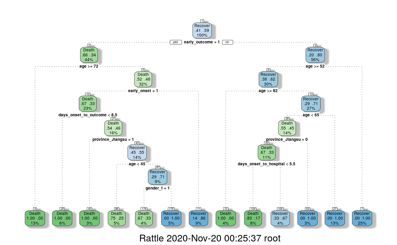
This randomly generated decision tree shows that cases with an early outcome were most likely to die when they were 68 or older, when they also had an early onset and when they were sick for fewer than 13 days. If a person was not among the first cases and was younger than 52, they had a good chance of recovering, but if they were 82 or older, they were more likely to die from the flu.
28.4.2 Feature Importance
Not all of the features I created will be equally important to the model. The decision tree already gave me an idea of which features might be most important but I also want to estimate feature importance using a Random Forest approach with repeated cross validation.
# prepare training scheme
control <- trainControl(method = "repeatedcv", number = 10, repeats = 10)

# train the model
set.seed(27)
model <- train(outcome ~ ., data = train_data, method = "rf",
               preProcess = NULL, trControl = control)

# estimate variable importance
importance <- varImp(model, scale=TRUE)
from <- c("age", "hospital1", "gender_f1", "province_Jiangsu1",
          "province_Shanghai1", "province_Zhejiang1", "province_other1",
          "days_onset_to_outcome", "days_onset_to_hospital", "early_onset1",
          "early_outcome1" )

to <- c("Age", "Hospital", "Female", "Jiangsu", "Shanghai", "Zhejiang",
        "Other province", "Days onset to outcome", "Days onset to hospital",
        "Early onset", "Early outcome" )

importance_df_1 <- importance$importance
importance_df_1$group <- rownames(importance_df_1)

importance_df_1$group <- mapvalues(importance_df_1$group,
                                           from = from,
                                           to = to)
f = importance_df_1[order(importance_df_1$Overall, decreasing = FALSE), "group"]

importance_df_2 <- importance_df_1
importance_df_2$Overall <- 0

importance_df <- rbind(importance_df_1, importance_df_2)

# setting factor levels
importance_df <- within(importance_df, group <- factor(group, levels = f))
importance_df_1 <- within(importance_df_1, group <- factor(group, levels = f))

ggplot() +
  geom_point(data = importance_df_1, aes(x = Overall, y = group,
                                         color = group), size = 2) +
  geom_path(data = importance_df, aes(x = Overall, y = group, color = group,
                                      group = group), size = 1) +
  scale_color_manual(values = rep(brewer.pal(1, "Set1")[1], 11)) +
  my_theme() +
  theme(legend.position = "none",
        axis.text.x = element_text(angle = 0, vjust = 0.5, hjust = 0.5)) +
  labs(
    x = "Importance",
    y = "",
    title = "2013 Influenza A H7N9 cases in China",
    subtitle = "Scaled feature importance",
    caption = "\nDetermined with Random Forest and
    repeated cross validation (10 repeats, 10 times)"
  )
#> Warning in brewer.pal(1, "Set1"): minimal value for n is 3, returning requested palette with 3 different levels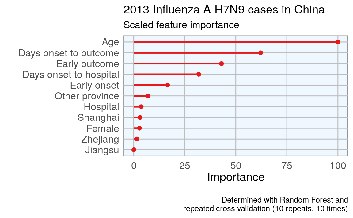
This tells me that age is the most important determining factor for predicting disease outcome, followed by days between onset an outcome, early outcome and days between onset and hospitalization.
28.4.3 Feature Plot
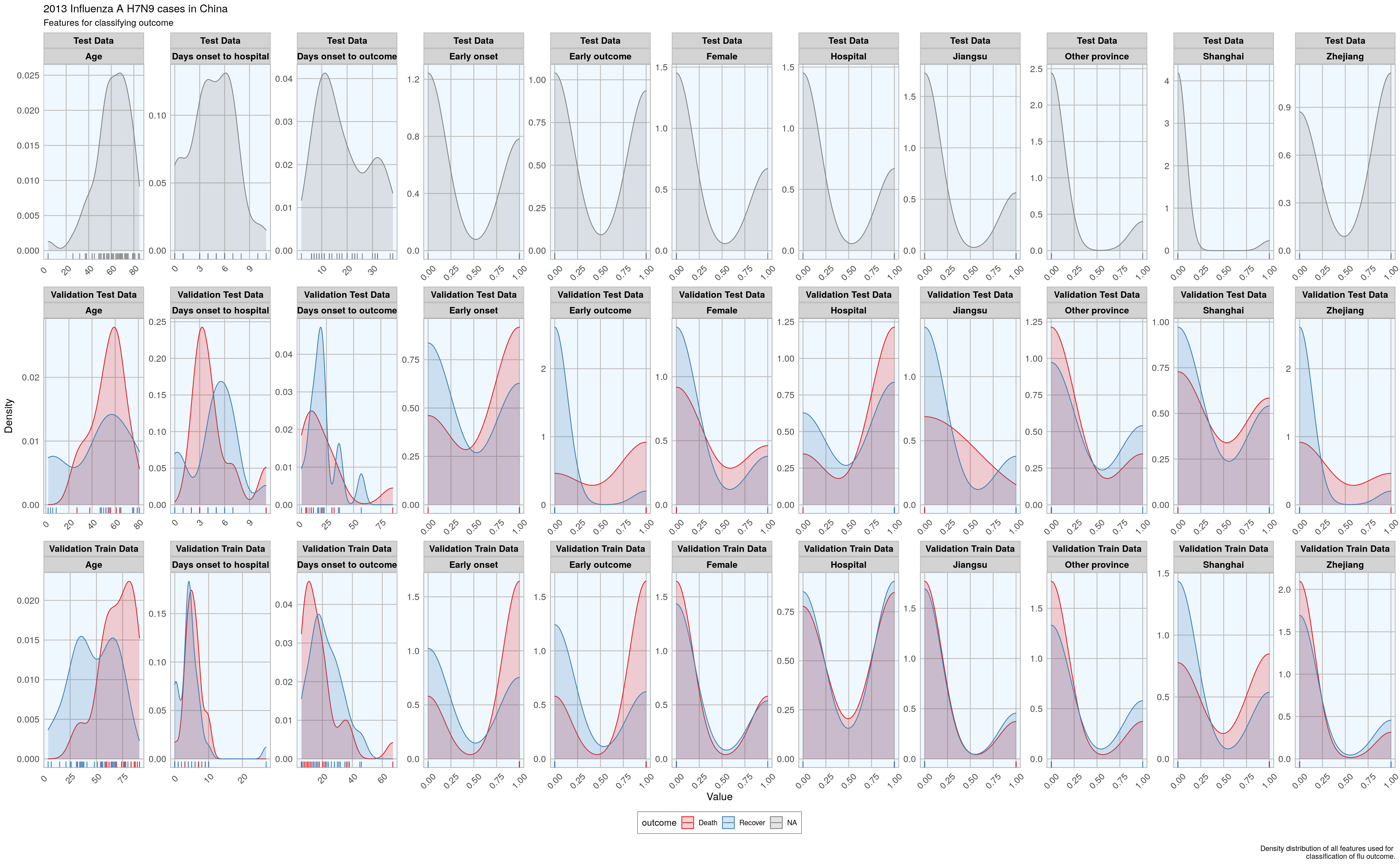
Before I start actually building models, I want to check whether the distribution of feature values is comparable between training, validation and test datasets.
# tidy dataframe of 11 variables for plotting features for all datasets
# dataset_complete: 136x12. test + val_train + val_test
dataset_complete_gather <- dataset_complete %>%
  mutate(set = ifelse(rownames(dataset_complete) %in% rownames(test_data),
                      "Test Data",
               ifelse(rownames(dataset_complete) %in% rownames(val_train_data),
                      "Validation Train Data",
               ifelse(rownames(dataset_complete) %in% rownames(val_test_data),
                      "Validation Test Data", "NA"))),
         case_ID = rownames(.)) %>%
  gather(group, value, age:early_outcome)
#> Warning: attributes are not identical across measure variables;
#> they will be dropped

# map values in group to more readable
from <- c("age", "hospital", "gender_f", "province_Jiangsu", "province_Shanghai",
          "province_Zhejiang", "province_other", "days_onset_to_outcome",
          "days_onset_to_hospital", "early_onset",  "early_outcome" )
to <- c("Age", "Hospital", "Female", "Jiangsu", "Shanghai", "Zhejiang",
        "Other province", "Days onset to outcome", "Days onset to hospital",
        "Early onset", "Early outcome" )
dataset_complete_gather$group <- mapvalues(dataset_complete_gather$group,
                      from = from,
                      to = to)
28.4.4 Plot distribution of features in each dataset
# plot features all datasets
ggplot(data = dataset_complete_gather,
       aes(x = as.numeric(value), fill = outcome, color = outcome)) +
  geom_density(alpha = 0.2) +
  geom_rug() +
  scale_color_brewer(palette="Set1", na.value = "grey50") +
  scale_fill_brewer(palette="Set1", na.value = "grey50") +
  my_theme() +
  facet_wrap(set ~ group, ncol = 11, scales = "free") +
  labs(
    x = "Value",
    y = "Density",
    title = "2013 Influenza A H7N9 cases in China",
    subtitle = "Features for classifying outcome",
    caption = "\nDensity distribution of all features used for
    classification of flu outcome."
  )
28.4.5 Plot 3 features vs outcome, all datasets
# plot three groups vs outcome
ggplot(subset(dataset_complete_gather,
              group == "Age" |
              group == "Days onset to hospital" |
              group == "Days onset to outcome"),
       aes(x=outcome, y=as.numeric(value), fill=set)) +
  geom_boxplot() +
  my_theme() +
  scale_fill_brewer(palette="Set1", type = "div ") +
  facet_wrap( ~ group, ncol = 3, scales = "free") +
  labs(
    fill = "",
    x = "Outcome",
    y = "Value",
    title = "2013 Influenza A H7N9 cases in China",
    subtitle = "Features for classifying outcome",
    caption = "\nBoxplot of the features age, days from onset to
    hospitalisation and days from onset to outcome."
  )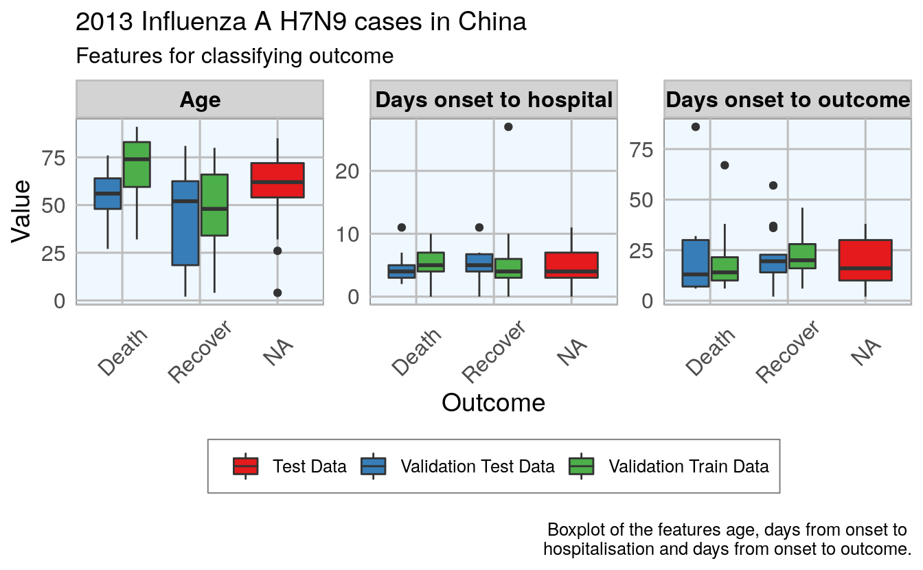
Luckily, the distributions looks reasonably similar between the validation and test data, except for a few outliers.
28.5 Comparing Machine Learning algorithms
Before I try to predict the outcome of the unknown cases, I am testing the models’ accuracy with the validation datasets on a couple of algorithms. I have chosen only a few more well known algorithms, but caret implements many more.
I have chosen to not do any preprocessing because I was worried that the different data distributions with continuous variables (e.g. age) and binary variables (i.e. 0, 1 classification of e.g. hospitalisation) would lead to problems.
- Random Forest
- GLM net
- k-Nearest Neighbors
- Penalized Discriminant Analysis
- Stabilized Linear Discriminant Analysis
- Nearest Shrunken Centroids
- Single C5.0 Tree
- Partial Least Squares
train_control <- trainControl(method = "repeatedcv",
                              number = 10,
                              repeats = 10,
                              verboseIter = FALSE)
28.5.1 Random Forest
Random Forests predictions are based on the generation of multiple classification trees. This model classified 14 out of 23 cases correctly.
set.seed(27)
model_rf <- caret::train(outcome ~ .,
                             data = val_train_data,
                             method = "rf",
                             preProcess = NULL,
                             trControl = train_control)
model_rf
#> Random Forest
#>
#> 56 samples
#> 11 predictors
#>  2 classes: 'Death', 'Recover'
#>
#> No pre-processing
#> Resampling: Cross-Validated (10 fold, repeated 10 times)
#> Summary of sample sizes: 51, 49, 50, 51, 49, 51, ...
#> Resampling results across tuning parameters:
#>
#>   mtry  Accuracy  Kappa
#>    2    0.687     0.340
#>    6    0.732     0.432
#>   11    0.726     0.423
#>
#> Accuracy was used to select the optimal model using the largest value.
#> The final value used for the model was mtry = 6.
confusionMatrix(predict(model_rf, val_test_data[, -1]), val_test_data$outcome)
#> Confusion Matrix and Statistics
#>
#>           Reference
#> Prediction Death Recover
#>    Death       3       0
#>    Recover     6      14
#>
#>                Accuracy : 0.739
#>                  95% CI : (0.516, 0.898)
#>     No Information Rate : 0.609
#>     P-Value [Acc > NIR] : 0.1421
#>
#>                   Kappa : 0.378
#>
#>  Mcnemar's Test P-Value : 0.0412
#>
#>             Sensitivity : 0.333
#>             Specificity : 1.000
#>          Pos Pred Value : 1.000
#>          Neg Pred Value : 0.700
#>              Prevalence : 0.391
#>          Detection Rate : 0.130
#>    Detection Prevalence : 0.130
#>       Balanced Accuracy : 0.667
#>
#>        'Positive' Class : Death
#>
28.5.2 GLM net
Lasso or elastic net regularization for generalized linear model regression are based on linear regression models and is useful when we have feature correlation in our model.
This model classified 13 out of 23 cases correctly.
set.seed(27)
model_glmnet <- caret::train(outcome ~ .,
                             data = val_train_data,
                             method = "glmnet",
                             preProcess = NULL,
                             trControl = train_control)
model_glmnet
#> glmnet
#>
#> 56 samples
#> 11 predictors
#>  2 classes: 'Death', 'Recover'
#>
#> No pre-processing
#> Resampling: Cross-Validated (10 fold, repeated 10 times)
#> Summary of sample sizes: 51, 49, 50, 51, 49, 51, ...
#> Resampling results across tuning parameters:
#>
#>   alpha  lambda    Accuracy  Kappa
#>   0.10   0.000491  0.671     0.324
#>   0.10   0.004909  0.669     0.318
#>   0.10   0.049093  0.680     0.339
#>   0.55   0.000491  0.671     0.324
#>   0.55   0.004909  0.671     0.322
#>   0.55   0.049093  0.695     0.365
#>   1.00   0.000491  0.671     0.324
#>   1.00   0.004909  0.672     0.326
#>   1.00   0.049093  0.714     0.414
#>
#> Accuracy was used to select the optimal model using the largest value.
#> The final values used for the model were alpha = 1 and lambda = 0.0491.
confusionMatrix(predict(model_glmnet, val_test_data[, -1]), val_test_data$outcome)
#> Confusion Matrix and Statistics
#>
#>           Reference
#> Prediction Death Recover
#>    Death       3       2
#>    Recover     6      12
#>
#>                Accuracy : 0.652
#>                  95% CI : (0.427, 0.836)
#>     No Information Rate : 0.609
#>     P-Value [Acc > NIR] : 0.422
#>
#>                   Kappa : 0.207
#>
#>  Mcnemar's Test P-Value : 0.289
#>
#>             Sensitivity : 0.333
#>             Specificity : 0.857
#>          Pos Pred Value : 0.600
#>          Neg Pred Value : 0.667
#>              Prevalence : 0.391
#>          Detection Rate : 0.130
#>    Detection Prevalence : 0.217
#>       Balanced Accuracy : 0.595
#>
#>        'Positive' Class : Death
#>
28.5.3 k-Nearest Neighbors
k-nearest neighbors predicts based on point distances with predefined constants. This model classified 14 out of 23 cases correctly.
set.seed(27)
model_kknn <- caret::train(outcome ~ .,
                             data = val_train_data,
                             method = "kknn",
                             preProcess = NULL,
                             trControl = train_control)
model_kknn
#> k-Nearest Neighbors
#>
#> 56 samples
#> 11 predictors
#>  2 classes: 'Death', 'Recover'
#>
#> No pre-processing
#> Resampling: Cross-Validated (10 fold, repeated 10 times)
#> Summary of sample sizes: 51, 49, 50, 51, 49, 51, ...
#> Resampling results across tuning parameters:
#>
#>   kmax  Accuracy  Kappa
#>   5     0.666     0.313
#>   7     0.653     0.274
#>   9     0.648     0.263
#>
#> Tuning parameter 'distance' was held constant at a value of 2
#> Tuning parameter 'kernel' was held constant at a value of optimal
#> Accuracy was used to select the optimal model using the largest value.
#> The final values used for the model were kmax = 5, distance = 2 and kernel = optimal.
confusionMatrix(predict(model_kknn, val_test_data[, -1]), val_test_data$outcome)
#> Confusion Matrix and Statistics
#>
#>           Reference
#> Prediction Death Recover
#>    Death       5       3
#>    Recover     4      11
#>
#>                Accuracy : 0.696
#>                  95% CI : (0.471, 0.868)
#>     No Information Rate : 0.609
#>     P-Value [Acc > NIR] : 0.264
#>
#>                   Kappa : 0.348
#>
#>  Mcnemar's Test P-Value : 1.000
#>
#>             Sensitivity : 0.556
#>             Specificity : 0.786
#>          Pos Pred Value : 0.625
#>          Neg Pred Value : 0.733
#>              Prevalence : 0.391
#>          Detection Rate : 0.217
#>    Detection Prevalence : 0.348
#>       Balanced Accuracy : 0.671
#>
#>        'Positive' Class : Death
#>
28.5.4 Penalized Discriminant Analysis
Penalized Discriminant Analysis is the penalized linear discriminant analysis and is also useful for when we have highly correlated features. This model classified 14 out of 23 cases correctly.
set.seed(27)
model_pda <- caret::train(outcome ~ .,
                             data = val_train_data,
                             method = "pda",
                             preProcess = NULL,
                             trControl = train_control)
model_pda
#> Penalized Discriminant Analysis
#>
#> 56 samples
#> 11 predictors
#>  2 classes: 'Death', 'Recover'
#>
#> No pre-processing
#> Resampling: Cross-Validated (10 fold, repeated 10 times)
#> Summary of sample sizes: 51, 49, 50, 51, 49, 51, ...
#> Resampling results across tuning parameters:
#>
#>   lambda  Accuracy  Kappa
#>   0e+00     NaN       NaN
#>   1e-04   0.681     0.343
#>   1e-01   0.681     0.343
#>
#> Accuracy was used to select the optimal model using the largest value.
#> The final value used for the model was lambda = 1e-04.
confusionMatrix(predict(model_pda, val_test_data[, -1]), val_test_data$outcome)
#> Confusion Matrix and Statistics
#>
#>           Reference
#> Prediction Death Recover
#>    Death       3       2
#>    Recover     6      12
#>
#>                Accuracy : 0.652
#>                  95% CI : (0.427, 0.836)
#>     No Information Rate : 0.609
#>     P-Value [Acc > NIR] : 0.422
#>
#>                   Kappa : 0.207
#>
#>  Mcnemar's Test P-Value : 0.289
#>
#>             Sensitivity : 0.333
#>             Specificity : 0.857
#>          Pos Pred Value : 0.600
#>          Neg Pred Value : 0.667
#>              Prevalence : 0.391
#>          Detection Rate : 0.130
#>    Detection Prevalence : 0.217
#>       Balanced Accuracy : 0.595
#>
#>        'Positive' Class : Death
#>
28.5.5 Stabilized Linear Discriminant Analysis
Stabilized Linear Discriminant Analysis is designed for high-dimensional data and correlated co-variables. This model classified 15 out of 23 cases correctly.
set.seed(27)
model_slda <- caret::train(outcome ~ .,
                             data = val_train_data,
                             method = "slda",
                             preProcess = NULL,
                             trControl = train_control)
model_slda
#> Stabilized Linear Discriminant Analysis
#>
#> 56 samples
#> 11 predictors
#>  2 classes: 'Death', 'Recover'
#>
#> No pre-processing
#> Resampling: Cross-Validated (10 fold, repeated 10 times)
#> Summary of sample sizes: 51, 49, 50, 51, 49, 51, ...
#> Resampling results:
#>
#>   Accuracy  Kappa
#>   0.682     0.358
confusionMatrix(predict(model_slda, val_test_data[, -1]), val_test_data$outcome)
#> Confusion Matrix and Statistics
#>
#>           Reference
#> Prediction Death Recover
#>    Death       3       3
#>    Recover     6      11
#>
#>                Accuracy : 0.609
#>                  95% CI : (0.385, 0.803)
#>     No Information Rate : 0.609
#>     P-Value [Acc > NIR] : 0.590
#>
#>                   Kappa : 0.127
#>
#>  Mcnemar's Test P-Value : 0.505
#>
#>             Sensitivity : 0.333
#>             Specificity : 0.786
#>          Pos Pred Value : 0.500
#>          Neg Pred Value : 0.647
#>              Prevalence : 0.391
#>          Detection Rate : 0.130
#>    Detection Prevalence : 0.261
#>       Balanced Accuracy : 0.560
#>
#>        'Positive' Class : Death
#>
28.5.6 Nearest Shrunken Centroids
Nearest Shrunken Centroids computes a standardized centroid for each class and shrinks each centroid toward the overall centroid for all classes. This model classified 15 out of 23 cases correctly.
set.seed(27)
model_pam <- caret::train(outcome ~ .,
                             data = val_train_data,
                             method = "pam",
                             preProcess = NULL,
                             trControl = train_control)
#> 12345678910111213141516171819202122232425262728293011111111111111111111111111111111111111111111111111111111111111111111111111111111111111111111111111111
model_pam
#> Nearest Shrunken Centroids
#>
#> 56 samples
#> 11 predictors
#>  2 classes: 'Death', 'Recover'
#>
#> No pre-processing
#> Resampling: Cross-Validated (10 fold, repeated 10 times)
#> Summary of sample sizes: 51, 49, 50, 51, 49, 51, ...
#> Resampling results across tuning parameters:
#>
#>   threshold  Accuracy  Kappa
#>   0.142      0.709     0.416
#>   2.065      0.714     0.382
#>   3.987      0.590     0.000
#>
#> Accuracy was used to select the optimal model using the largest value.
#> The final value used for the model was threshold = 2.06.
confusionMatrix(predict(model_pam, val_test_data[, -1]), val_test_data$outcome)
#> Confusion Matrix and Statistics
#>
#>           Reference
#> Prediction Death Recover
#>    Death       1       3
#>    Recover     8      11
#>
#>                Accuracy : 0.522
#>                  95% CI : (0.306, 0.732)
#>     No Information Rate : 0.609
#>     P-Value [Acc > NIR] : 0.857
#>
#>                   Kappa : -0.115
#>
#>  Mcnemar's Test P-Value : 0.228
#>
#>             Sensitivity : 0.1111
#>             Specificity : 0.7857
#>          Pos Pred Value : 0.2500
#>          Neg Pred Value : 0.5789
#>              Prevalence : 0.3913
#>          Detection Rate : 0.0435
#>    Detection Prevalence : 0.1739
#>       Balanced Accuracy : 0.4484
#>
#>        'Positive' Class : Death
#>
28.5.7 Single C5.0 Tree
C5.0 is another tree-based modeling algorithm. This model classified 15 out of 23 cases correctly.
set.seed(27)
model_C5.0Tree <- caret::train(outcome ~ .,
                             data = val_train_data,
                             method = "C5.0Tree",
                             preProcess = NULL,
                             trControl = train_control)
model_C5.0Tree
#> Single C5.0 Tree
#>
#> 56 samples
#> 11 predictors
#>  2 classes: 'Death', 'Recover'
#>
#> No pre-processing
#> Resampling: Cross-Validated (10 fold, repeated 10 times)
#> Summary of sample sizes: 51, 49, 50, 51, 49, 51, ...
#> Resampling results:
#>
#>   Accuracy  Kappa
#>   0.696     0.359
confusionMatrix(predict(model_C5.0Tree, val_test_data[, -1]), val_test_data$outcome)
#> Confusion Matrix and Statistics
#>
#>           Reference
#> Prediction Death Recover
#>    Death       4       1
#>    Recover     5      13
#>
#>                Accuracy : 0.739
#>                  95% CI : (0.516, 0.898)
#>     No Information Rate : 0.609
#>     P-Value [Acc > NIR] : 0.142
#>
#>                   Kappa : 0.405
#>
#>  Mcnemar's Test P-Value : 0.221
#>
#>             Sensitivity : 0.444
#>             Specificity : 0.929
#>          Pos Pred Value : 0.800
#>          Neg Pred Value : 0.722
#>              Prevalence : 0.391
#>          Detection Rate : 0.174
#>    Detection Prevalence : 0.217
#>       Balanced Accuracy : 0.687
#>
#>        'Positive' Class : Death
#>
28.5.8 Partial Least Squares
modeling with correlated features. This model classified 15 out of 23 cases correctly.
set.seed(27)
model_pls <- caret::train(outcome ~ .,
                             data = val_train_data,
                             method = "pls",
                             preProcess = NULL,
                             trControl = train_control)
model_pls
#> Partial Least Squares
#>
#> 56 samples
#> 11 predictors
#>  2 classes: 'Death', 'Recover'
#>
#> No pre-processing
#> Resampling: Cross-Validated (10 fold, repeated 10 times)
#> Summary of sample sizes: 51, 49, 50, 51, 49, 51, ...
#> Resampling results across tuning parameters:
#>
#>   ncomp  Accuracy  Kappa
#>   1      0.663     0.315
#>   2      0.676     0.341
#>   3      0.691     0.376
#>
#> Accuracy was used to select the optimal model using the largest value.
#> The final value used for the model was ncomp = 3.
confusionMatrix(predict(model_pls, val_test_data[, -1]), val_test_data$outcome)
#> Confusion Matrix and Statistics
#>
#>           Reference
#> Prediction Death Recover
#>    Death       2       3
#>    Recover     7      11
#>
#>                Accuracy : 0.565
#>                  95% CI : (0.345, 0.768)
#>     No Information Rate : 0.609
#>     P-Value [Acc > NIR] : 0.742
#>
#>                   Kappa : 0.009
#>
#>  Mcnemar's Test P-Value : 0.343
#>
#>             Sensitivity : 0.222
#>             Specificity : 0.786
#>          Pos Pred Value : 0.400
#>          Neg Pred Value : 0.611
#>              Prevalence : 0.391
#>          Detection Rate : 0.087
#>    Detection Prevalence : 0.217
#>       Balanced Accuracy : 0.504
#>
#>        'Positive' Class : Death
#>
28.6 Comparing accuracy of models
All models were similarly accurate.
28.6.1 Summary Accuracy and Kappa
# Create a list of models
models <- list(rf       = model_rf,
               glmnet   = model_glmnet,
               kknn     = model_kknn,
               pda      = model_pda,
               slda     = model_slda,
               pam      = model_pam,
               C5.0Tree = model_C5.0Tree,
               pls      = model_pls)

# Resample the models
resample_results <- resamples(models)

# Generate a summary
summary(resample_results, metric = c("Kappa", "Accuracy"))
#>
#> Call:
#> summary.resamples(object = resample_results, metric = c("Kappa", "Accuracy"))
#>
#> Models: rf, glmnet, kknn, pda, slda, pam, C5.0Tree, pls
#> Number of resamples: 100
#>
#> Kappa
#>            Min. 1st Qu. Median  Mean 3rd Qu. Max. NA's
#> rf       -0.500   0.167  0.545 0.432   0.667    1    0
#> glmnet   -0.667   0.167  0.545 0.414   0.667    1    0
#> kknn     -0.667   0.125  0.333 0.313   0.615    1    0
#> pda      -0.667   0.142  0.333 0.343   0.615    1    0
#> slda     -0.667   0.167  0.367 0.358   0.615    1    0
#> pam      -0.667   0.167  0.545 0.382   0.571    1    0
#> C5.0Tree -0.667   0.167  0.333 0.359   0.615    1    0
#> pls      -0.667   0.167  0.333 0.376   0.667    1    0
#>
#> Accuracy
#>           Min. 1st Qu. Median  Mean 3rd Qu. Max. NA's
#> rf       0.333   0.600  0.800 0.732   0.833    1    0
#> glmnet   0.167   0.600  0.800 0.714   0.833    1    0
#> kknn     0.167   0.600  0.667 0.666   0.800    1    0
#> pda      0.167   0.593  0.667 0.681   0.800    1    0
#> slda     0.167   0.600  0.667 0.682   0.800    1    0
#> pam      0.200   0.600  0.800 0.714   0.800    1    0
#> C5.0Tree 0.167   0.600  0.667 0.696   0.800    1    0
#> pls      0.167   0.600  0.667 0.691   0.833    1    0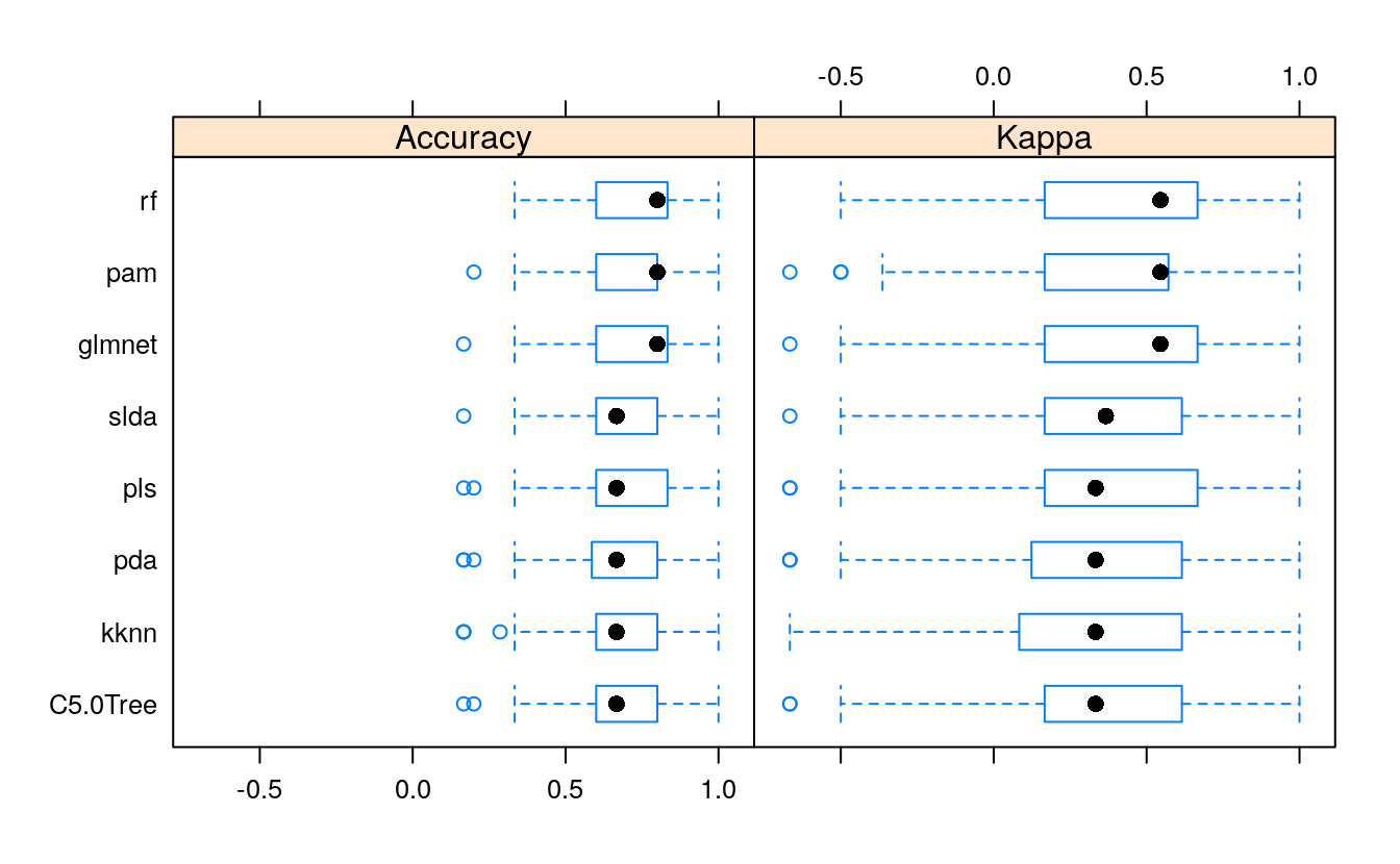
28.6.2 Combined results of predicting validation test samples
To compare the predictions from all models, I summed up the prediction probabilities for Death and Recovery from all models and calculated the log2 of the ratio between the summed probabilities for Recovery by the summed probabilities for Death. All cases with a log2 ratio bigger than 1.5 were defined as Recover, cases with a \(log2\) ratio below -1.5 were defined as Death, and the remaining cases were defined as uncertain.
results <- data.frame(
  randomForest = predict(model_rf, newdata = val_test_data[, -1], type="prob"),
  glmnet = predict(model_glmnet, newdata = val_test_data[, -1], type="prob"),
  kknn = predict(model_kknn, newdata = val_test_data[, -1], type="prob"),
  pda = predict(model_pda, newdata = val_test_data[, -1], type="prob"),
  slda = predict(model_slda, newdata = val_test_data[, -1], type="prob"),
  pam = predict(model_pam, newdata = val_test_data[, -1], type="prob"),
  C5.0Tree = predict(model_C5.0Tree, newdata = val_test_data[, -1], type="prob"),
  pls = predict(model_pls, newdata = val_test_data[, -1], type="prob"))

results$sum_Death <- rowSums(results[, grep("Death", colnames(results))])
results$sum_Recover <- rowSums(results[, grep("Recover", colnames(results))])
results$log2_ratio <- log2(results$sum_Recover/results$sum_Death)
results$true_outcome <- val_test_data$outcome
results$pred_outcome <- ifelse(results$log2_ratio > 1.5, "Recover",
              ifelse(results$log2_ratio < -1.5, "Death", "uncertain"))
results$prediction <- ifelse(results$pred_outcome == results$true_outcome, "CORRECT",
              ifelse(results$pred_outcome == "uncertain", "uncertain", "wrong"))
results[, -c(1:16)]
#>          sum_Death sum_Recover log2_ratio true_outcome pred_outcome prediction
#> case_10      4.237        3.76    -0.1709        Death    uncertain  uncertain
#> case_11      5.181        2.82    -0.8778        Death    uncertain  uncertain
#> case_116     2.412        5.59     1.2123      Recover    uncertain  uncertain
#> case_12      5.219        2.78    -0.9085        Death    uncertain  uncertain
#> case_121     2.356        5.64     1.2606        Death    uncertain  uncertain
#> case_127     0.694        7.31     3.3972      Recover      Recover    CORRECT
#> case_131     0.685        7.31     3.4164      Recover      Recover    CORRECT
#> case_133     0.649        7.35     3.5024      Recover      Recover    CORRECT
#> case_135     2.027        5.97     1.5589        Death      Recover      wrong
#> case_2       2.161        5.84     1.4337        Death    uncertain  uncertain
#> case_20      3.144        4.86     0.6272      Recover    uncertain  uncertain
#> case_30      4.493        3.51    -0.3576      Recover    uncertain  uncertain
#> case_45      2.594        5.41     1.0590        Death    uncertain  uncertain
#> case_5       3.019        4.98     0.7227      Recover    uncertain  uncertain
#> case_55      3.925        4.08     0.0543      Recover    uncertain  uncertain
#> case_59      1.894        6.11     1.6886      Recover      Recover    CORRECT
#> case_72      2.545        5.46     1.1002      Recover    uncertain  uncertain
#> case_74      2.339        5.66     1.2748      Recover    uncertain  uncertain
#> case_77      0.845        7.15     3.0819      Recover      Recover    CORRECT
#> case_8       2.237        5.76     1.3650        Death    uncertain  uncertain
#> case_89      1.712        6.29     1.8772      Recover      Recover    CORRECT
#> case_97      2.959        5.04     0.7687      Recover    uncertain  uncertain
#> case_98      4.798        3.20    -0.5833        Death    uncertain  uncertain
All predictions based on all models were either correct or uncertain.
28.7 Predicting unknown outcomes
The above models will now be used to predict the outcome of cases with unknown fate.
train_control <- trainControl(method = "repeatedcv",
                              number = 10,
                              repeats = 10,
                              verboseIter = FALSE)

set.seed(27)
model_rf <- caret::train(outcome ~ .,
                             data = train_data,
                             method = "rf",
                             preProcess = NULL,
                             trControl = train_control)
model_glmnet <- caret::train(outcome ~ .,
                             data = train_data,
                             method = "glmnet",
                             preProcess = NULL,
                             trControl = train_control)
model_kknn <- caret::train(outcome ~ .,
                             data = train_data,
                             method = "kknn",
                             preProcess = NULL,
                             trControl = train_control)
model_pda <- caret::train(outcome ~ .,
                             data = train_data,
                             method = "pda",
                             preProcess = NULL,
                             trControl = train_control)
#> Warning: predictions failed for Fold01.Rep01: lambda=0e+00 Error in mindist[l] <- ndist[l] :
#>   NAs are not allowed in subscripted assignments
#> Warning: predictions failed for Fold02.Rep01: lambda=0e+00 Error in mindist[l] <- ndist[l] :
#>   NAs are not allowed in subscripted assignments
#> Warning: predictions failed for Fold03.Rep01: lambda=0e+00 Error in mindist[l] <- ndist[l] :
#>   NAs are not allowed in subscripted assignments
#> Warning: predictions failed for Fold04.Rep01: lambda=0e+00 Error in mindist[l] <- ndist[l] :
#>   NAs are not allowed in subscripted assignments
#> Warning: predictions failed for Fold05.Rep01: lambda=0e+00 Error in mindist[l] <- ndist[l] :
#>   NAs are not allowed in subscripted assignments
#> Warning: predictions failed for Fold06.Rep01: lambda=0e+00 Error in mindist[l] <- ndist[l] :
#>   NAs are not allowed in subscripted assignments
#> Warning: predictions failed for Fold07.Rep01: lambda=0e+00 Error in mindist[l] <- ndist[l] :
#>   NAs are not allowed in subscripted assignments
#> Warning: predictions failed for Fold08.Rep01: lambda=0e+00 Error in mindist[l] <- ndist[l] :
#>   NAs are not allowed in subscripted assignments
#> Warning: predictions failed for Fold09.Rep01: lambda=0e+00 Error in mindist[l] <- ndist[l] :
#>   NAs are not allowed in subscripted assignments
#> Warning: predictions failed for Fold10.Rep01: lambda=0e+00 Error in mindist[l] <- ndist[l] :
#>   NAs are not allowed in subscripted assignments
#> Warning: predictions failed for Fold01.Rep02: lambda=0e+00 Error in mindist[l] <- ndist[l] :
#>   NAs are not allowed in subscripted assignments
#> Warning: predictions failed for Fold02.Rep02: lambda=0e+00 Error in mindist[l] <- ndist[l] :
#>   NAs are not allowed in subscripted assignments
#> Warning: predictions failed for Fold03.Rep02: lambda=0e+00 Error in mindist[l] <- ndist[l] :
#>   NAs are not allowed in subscripted assignments
#> Warning: predictions failed for Fold04.Rep02: lambda=0e+00 Error in mindist[l] <- ndist[l] :
#>   NAs are not allowed in subscripted assignments
#> Warning: predictions failed for Fold05.Rep02: lambda=0e+00 Error in mindist[l] <- ndist[l] :
#>   NAs are not allowed in subscripted assignments
#> Warning: predictions failed for Fold06.Rep02: lambda=0e+00 Error in mindist[l] <- ndist[l] :
#>   NAs are not allowed in subscripted assignments
#> Warning: predictions failed for Fold07.Rep02: lambda=0e+00 Error in mindist[l] <- ndist[l] :
#>   NAs are not allowed in subscripted assignments
#> Warning: predictions failed for Fold08.Rep02: lambda=0e+00 Error in mindist[l] <- ndist[l] :
#>   NAs are not allowed in subscripted assignments
#> Warning: predictions failed for Fold09.Rep02: lambda=0e+00 Error in mindist[l] <- ndist[l] :
#>   NAs are not allowed in subscripted assignments
#> Warning: predictions failed for Fold10.Rep02: lambda=0e+00 Error in mindist[l] <- ndist[l] :
#>   NAs are not allowed in subscripted assignments
#> Warning: predictions failed for Fold01.Rep03: lambda=0e+00 Error in mindist[l] <- ndist[l] :
#>   NAs are not allowed in subscripted assignments
#> Warning: predictions failed for Fold02.Rep03: lambda=0e+00 Error in mindist[l] <- ndist[l] :
#>   NAs are not allowed in subscripted assignments
#> Warning: predictions failed for Fold03.Rep03: lambda=0e+00 Error in mindist[l] <- ndist[l] :
#>   NAs are not allowed in subscripted assignments
#> Warning: predictions failed for Fold04.Rep03: lambda=0e+00 Error in mindist[l] <- ndist[l] :
#>   NAs are not allowed in subscripted assignments
#> Warning: predictions failed for Fold05.Rep03: lambda=0e+00 Error in mindist[l] <- ndist[l] :
#>   NAs are not allowed in subscripted assignments
#> Warning: predictions failed for Fold06.Rep03: lambda=0e+00 Error in mindist[l] <- ndist[l] :
#>   NAs are not allowed in subscripted assignments
#> Warning: predictions failed for Fold07.Rep03: lambda=0e+00 Error in mindist[l] <- ndist[l] :
#>   NAs are not allowed in subscripted assignments
#> Warning: predictions failed for Fold08.Rep03: lambda=0e+00 Error in mindist[l] <- ndist[l] :
#>   NAs are not allowed in subscripted assignments
#> Warning: predictions failed for Fold09.Rep03: lambda=0e+00 Error in mindist[l] <- ndist[l] :
#>   NAs are not allowed in subscripted assignments
#> Warning: predictions failed for Fold10.Rep03: lambda=0e+00 Error in mindist[l] <- ndist[l] :
#>   NAs are not allowed in subscripted assignments
#> Warning: predictions failed for Fold01.Rep04: lambda=0e+00 Error in mindist[l] <- ndist[l] :
#>   NAs are not allowed in subscripted assignments
#> Warning: predictions failed for Fold02.Rep04: lambda=0e+00 Error in mindist[l] <- ndist[l] :
#>   NAs are not allowed in subscripted assignments
#> Warning: predictions failed for Fold03.Rep04: lambda=0e+00 Error in mindist[l] <- ndist[l] :
#>   NAs are not allowed in subscripted assignments
#> Warning: predictions failed for Fold04.Rep04: lambda=0e+00 Error in mindist[l] <- ndist[l] :
#>   NAs are not allowed in subscripted assignments
#> Warning: predictions failed for Fold05.Rep04: lambda=0e+00 Error in mindist[l] <- ndist[l] :
#>   NAs are not allowed in subscripted assignments
#> Warning: predictions failed for Fold06.Rep04: lambda=0e+00 Error in mindist[l] <- ndist[l] :
#>   NAs are not allowed in subscripted assignments
#> Warning: predictions failed for Fold07.Rep04: lambda=0e+00 Error in mindist[l] <- ndist[l] :
#>   NAs are not allowed in subscripted assignments
#> Warning: predictions failed for Fold08.Rep04: lambda=0e+00 Error in mindist[l] <- ndist[l] :
#>   NAs are not allowed in subscripted assignments
#> Warning: predictions failed for Fold09.Rep04: lambda=0e+00 Error in mindist[l] <- ndist[l] :
#>   NAs are not allowed in subscripted assignments
#> Warning: predictions failed for Fold10.Rep04: lambda=0e+00 Error in mindist[l] <- ndist[l] :
#>   NAs are not allowed in subscripted assignments
#> Warning: predictions failed for Fold01.Rep05: lambda=0e+00 Error in mindist[l] <- ndist[l] :
#>   NAs are not allowed in subscripted assignments
#> Warning: predictions failed for Fold02.Rep05: lambda=0e+00 Error in mindist[l] <- ndist[l] :
#>   NAs are not allowed in subscripted assignments
#> Warning: predictions failed for Fold03.Rep05: lambda=0e+00 Error in mindist[l] <- ndist[l] :
#>   NAs are not allowed in subscripted assignments
#> Warning: predictions failed for Fold04.Rep05: lambda=0e+00 Error in mindist[l] <- ndist[l] :
#>   NAs are not allowed in subscripted assignments
#> Warning: predictions failed for Fold05.Rep05: lambda=0e+00 Error in mindist[l] <- ndist[l] :
#>   NAs are not allowed in subscripted assignments
#> Warning: predictions failed for Fold06.Rep05: lambda=0e+00 Error in mindist[l] <- ndist[l] :
#>   NAs are not allowed in subscripted assignments
#> Warning: predictions failed for Fold07.Rep05: lambda=0e+00 Error in mindist[l] <- ndist[l] :
#>   NAs are not allowed in subscripted assignments
#> Warning: predictions failed for Fold08.Rep05: lambda=0e+00 Error in mindist[l] <- ndist[l] :
#>   NAs are not allowed in subscripted assignments
#> Warning: predictions failed for Fold09.Rep05: lambda=0e+00 Error in mindist[l] <- ndist[l] :
#>   NAs are not allowed in subscripted assignments
#> Warning: predictions failed for Fold10.Rep05: lambda=0e+00 Error in mindist[l] <- ndist[l] :
#>   NAs are not allowed in subscripted assignments
#> Warning: predictions failed for Fold01.Rep06: lambda=0e+00 Error in mindist[l] <- ndist[l] :
#>   NAs are not allowed in subscripted assignments
#> Warning: predictions failed for Fold02.Rep06: lambda=0e+00 Error in mindist[l] <- ndist[l] :
#>   NAs are not allowed in subscripted assignments
#> Warning: predictions failed for Fold03.Rep06: lambda=0e+00 Error in mindist[l] <- ndist[l] :
#>   NAs are not allowed in subscripted assignments
#> Warning: predictions failed for Fold04.Rep06: lambda=0e+00 Error in mindist[l] <- ndist[l] :
#>   NAs are not allowed in subscripted assignments
#> Warning: predictions failed for Fold05.Rep06: lambda=0e+00 Error in mindist[l] <- ndist[l] :
#>   NAs are not allowed in subscripted assignments
#> Warning: predictions failed for Fold06.Rep06: lambda=0e+00 Error in mindist[l] <- ndist[l] :
#>   NAs are not allowed in subscripted assignments
#> Warning: predictions failed for Fold07.Rep06: lambda=0e+00 Error in mindist[l] <- ndist[l] :
#>   NAs are not allowed in subscripted assignments
#> Warning: predictions failed for Fold08.Rep06: lambda=0e+00 Error in mindist[l] <- ndist[l] :
#>   NAs are not allowed in subscripted assignments
#> Warning: predictions failed for Fold09.Rep06: lambda=0e+00 Error in mindist[l] <- ndist[l] :
#>   NAs are not allowed in subscripted assignments
#> Warning: predictions failed for Fold10.Rep06: lambda=0e+00 Error in mindist[l] <- ndist[l] :
#>   NAs are not allowed in subscripted assignments
#> Warning: predictions failed for Fold01.Rep07: lambda=0e+00 Error in mindist[l] <- ndist[l] :
#>   NAs are not allowed in subscripted assignments
#> Warning: predictions failed for Fold02.Rep07: lambda=0e+00 Error in mindist[l] <- ndist[l] :
#>   NAs are not allowed in subscripted assignments
#> Warning: predictions failed for Fold03.Rep07: lambda=0e+00 Error in mindist[l] <- ndist[l] :
#>   NAs are not allowed in subscripted assignments
#> Warning: predictions failed for Fold04.Rep07: lambda=0e+00 Error in mindist[l] <- ndist[l] :
#>   NAs are not allowed in subscripted assignments
#> Warning: predictions failed for Fold05.Rep07: lambda=0e+00 Error in mindist[l] <- ndist[l] :
#>   NAs are not allowed in subscripted assignments
#> Warning: predictions failed for Fold06.Rep07: lambda=0e+00 Error in mindist[l] <- ndist[l] :
#>   NAs are not allowed in subscripted assignments
#> Warning: predictions failed for Fold07.Rep07: lambda=0e+00 Error in mindist[l] <- ndist[l] :
#>   NAs are not allowed in subscripted assignments
#> Warning: predictions failed for Fold08.Rep07: lambda=0e+00 Error in mindist[l] <- ndist[l] :
#>   NAs are not allowed in subscripted assignments
#> Warning: predictions failed for Fold09.Rep07: lambda=0e+00 Error in mindist[l] <- ndist[l] :
#>   NAs are not allowed in subscripted assignments
#> Warning: predictions failed for Fold10.Rep07: lambda=0e+00 Error in mindist[l] <- ndist[l] :
#>   NAs are not allowed in subscripted assignments
#> Warning: predictions failed for Fold01.Rep08: lambda=0e+00 Error in mindist[l] <- ndist[l] :
#>   NAs are not allowed in subscripted assignments
#> Warning: predictions failed for Fold02.Rep08: lambda=0e+00 Error in mindist[l] <- ndist[l] :
#>   NAs are not allowed in subscripted assignments
#> Warning: predictions failed for Fold03.Rep08: lambda=0e+00 Error in mindist[l] <- ndist[l] :
#>   NAs are not allowed in subscripted assignments
#> Warning: predictions failed for Fold04.Rep08: lambda=0e+00 Error in mindist[l] <- ndist[l] :
#>   NAs are not allowed in subscripted assignments
#> Warning: predictions failed for Fold05.Rep08: lambda=0e+00 Error in mindist[l] <- ndist[l] :
#>   NAs are not allowed in subscripted assignments
#> Warning: predictions failed for Fold06.Rep08: lambda=0e+00 Error in mindist[l] <- ndist[l] :
#>   NAs are not allowed in subscripted assignments
#> Warning: predictions failed for Fold07.Rep08: lambda=0e+00 Error in mindist[l] <- ndist[l] :
#>   NAs are not allowed in subscripted assignments
#> Warning: predictions failed for Fold08.Rep08: lambda=0e+00 Error in mindist[l] <- ndist[l] :
#>   NAs are not allowed in subscripted assignments
#> Warning: predictions failed for Fold09.Rep08: lambda=0e+00 Error in mindist[l] <- ndist[l] :
#>   NAs are not allowed in subscripted assignments
#> Warning: predictions failed for Fold10.Rep08: lambda=0e+00 Error in mindist[l] <- ndist[l] :
#>   NAs are not allowed in subscripted assignments
#> Warning: predictions failed for Fold01.Rep09: lambda=0e+00 Error in mindist[l] <- ndist[l] :
#>   NAs are not allowed in subscripted assignments
#> Warning: predictions failed for Fold02.Rep09: lambda=0e+00 Error in mindist[l] <- ndist[l] :
#>   NAs are not allowed in subscripted assignments
#> Warning: predictions failed for Fold03.Rep09: lambda=0e+00 Error in mindist[l] <- ndist[l] :
#>   NAs are not allowed in subscripted assignments
#> Warning: predictions failed for Fold04.Rep09: lambda=0e+00 Error in mindist[l] <- ndist[l] :
#>   NAs are not allowed in subscripted assignments
#> Warning: predictions failed for Fold05.Rep09: lambda=0e+00 Error in mindist[l] <- ndist[l] :
#>   NAs are not allowed in subscripted assignments
#> Warning: predictions failed for Fold06.Rep09: lambda=0e+00 Error in mindist[l] <- ndist[l] :
#>   NAs are not allowed in subscripted assignments
#> Warning: predictions failed for Fold07.Rep09: lambda=0e+00 Error in mindist[l] <- ndist[l] :
#>   NAs are not allowed in subscripted assignments
#> Warning: predictions failed for Fold08.Rep09: lambda=0e+00 Error in mindist[l] <- ndist[l] :
#>   NAs are not allowed in subscripted assignments
#> Warning: predictions failed for Fold09.Rep09: lambda=0e+00 Error in mindist[l] <- ndist[l] :
#>   NAs are not allowed in subscripted assignments
#> Warning: predictions failed for Fold10.Rep09: lambda=0e+00 Error in mindist[l] <- ndist[l] :
#>   NAs are not allowed in subscripted assignments
#> Warning: predictions failed for Fold01.Rep10: lambda=0e+00 Error in mindist[l] <- ndist[l] :
#>   NAs are not allowed in subscripted assignments
#> Warning: predictions failed for Fold02.Rep10: lambda=0e+00 Error in mindist[l] <- ndist[l] :
#>   NAs are not allowed in subscripted assignments
#> Warning: predictions failed for Fold03.Rep10: lambda=0e+00 Error in mindist[l] <- ndist[l] :
#>   NAs are not allowed in subscripted assignments
#> Warning: predictions failed for Fold04.Rep10: lambda=0e+00 Error in mindist[l] <- ndist[l] :
#>   NAs are not allowed in subscripted assignments
#> Warning: predictions failed for Fold05.Rep10: lambda=0e+00 Error in mindist[l] <- ndist[l] :
#>   NAs are not allowed in subscripted assignments
#> Warning: predictions failed for Fold06.Rep10: lambda=0e+00 Error in mindist[l] <- ndist[l] :
#>   NAs are not allowed in subscripted assignments
#> Warning: predictions failed for Fold07.Rep10: lambda=0e+00 Error in mindist[l] <- ndist[l] :
#>   NAs are not allowed in subscripted assignments
#> Warning: predictions failed for Fold08.Rep10: lambda=0e+00 Error in mindist[l] <- ndist[l] :
#>   NAs are not allowed in subscripted assignments
#> Warning: predictions failed for Fold09.Rep10: lambda=0e+00 Error in mindist[l] <- ndist[l] :
#>   NAs are not allowed in subscripted assignments
#> Warning: predictions failed for Fold10.Rep10: lambda=0e+00 Error in mindist[l] <- ndist[l] :
#>   NAs are not allowed in subscripted assignments
#> Warning in nominalTrainWorkflow(x = x, y = y, wts = weights, info = trainInfo, : There were missing values in resampled performance measures.
#> Warning in train.default(x, y, weights = w, ...): missing values found in aggregated results
model_slda <- caret::train(outcome ~ .,
                             data = train_data,
                             method = "slda",
                             preProcess = NULL,
                             trControl = train_control)
model_pam <- caret::train(outcome ~ .,
                             data = train_data,
                             method = "pam",
                             preProcess = NULL,
                             trControl = train_control)
#> 12345678910111213141516171819202122232425262728293011111111111111111111111111111111111111111111111111111111111111111111111111111111111111111111111111111
model_C5.0Tree <- caret::train(outcome ~ .,
                             data = train_data,
                             method = "C5.0Tree",
                             preProcess = NULL,
                             trControl = train_control)
model_pls <- caret::train(outcome ~ .,
                             data = train_data,
                             method = "pls",
                             preProcess = NULL,
                             trControl = train_control)

models <- list(rf = model_rf,
               glmnet   = model_glmnet,
               kknn     = model_kknn,
               pda      = model_pda,
               slda     = model_slda,
               pam      = model_pam,
               C5.0Tree = model_C5.0Tree,
               pls      = model_pls)

# Resample the models
resample_results <- resamples(models)

bwplot(resample_results , metric = c("Kappa","Accuracy"))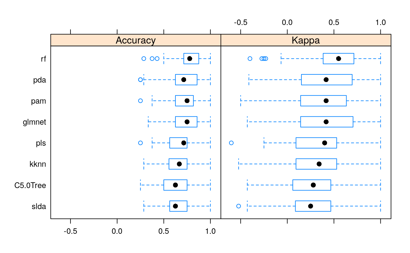
Here again, the accuracy is similar in all models.
28.7.1 Final results
The final results are calculated as described above.
results <- data.frame(
  randomForest = predict(model_rf, newdata = test_data, type="prob"),
  glmnet = predict(model_glmnet, newdata = test_data, type="prob"),
  kknn = predict(model_kknn, newdata = test_data, type="prob"),
  pda = predict(model_pda, newdata = test_data, type="prob"),
  slda = predict(model_slda, newdata = test_data, type="prob"),
  pam = predict(model_pam, newdata = test_data, type="prob"),
  C5.0Tree = predict(model_C5.0Tree, newdata = test_data, type="prob"),
  pls = predict(model_pls, newdata = test_data, type="prob"))

results$sum_Death <- rowSums(results[, grep("Death", colnames(results))])
results$sum_Recover <- rowSums(results[, grep("Recover", colnames(results))])
results$log2_ratio <- log2(results$sum_Recover/results$sum_Death)
results$predicted_outcome <- ifelse(results$log2_ratio > 1.5, "Recover",
                                    ifelse(results$log2_ratio < -1.5, "Death",
                                           "uncertain"))
results[, -c(1:16)]
#>          sum_Death sum_Recover log2_ratio predicted_outcome
#> case_100     1.854        6.15     1.7287           Recover
#> case_101     5.432        2.57    -1.0807         uncertain
#> case_102     2.806        5.19     0.8887         uncertain
#> case_103     2.342        5.66     1.2729         uncertain
#> case_104     1.744        6.26     1.8432           Recover
#> case_105     0.955        7.04     2.8828           Recover
#> case_108     4.489        3.51    -0.3543         uncertain
#> case_109     4.515        3.48    -0.3736         uncertain
#> case_110     2.411        5.59     1.2132         uncertain
#> case_112     2.632        5.37     1.0281         uncertain
#> case_113     2.198        5.80     1.4004         uncertain
#> case_114     3.339        4.66     0.4810         uncertain
#> case_115     1.112        6.89     2.6307           Recover
#> case_118     2.778        5.22     0.9109         uncertain
#> case_120     2.213        5.79     1.3868         uncertain
#> case_122     3.235        4.77     0.5590         uncertain
#> case_126     3.186        4.81     0.5952         uncertain
#> case_130     2.300        5.70     1.3091         uncertain
#> case_132     4.473        3.53    -0.3427         uncertain
#> case_136     3.281        4.72     0.5243         uncertain
#> case_15      2.270        5.73     1.3355         uncertain
#> case_16      2.820        5.18     0.8772         uncertain
#> case_22      4.779        3.22    -0.5689         uncertain
#> case_28      2.862        5.14     0.8445         uncertain
#> case_31      2.412        5.59     1.2117         uncertain
#> case_32      2.591        5.41     1.0616         uncertain
#> case_38      2.060        5.94     1.5280           Recover
#> case_39      4.749        3.25    -0.5466         uncertain
#> case_4       5.342        2.66    -1.0074         uncertain
#> case_40      6.550        1.45    -2.1750             Death
#> case_41      4.611        3.39    -0.4441         uncertain
#> case_42      5.570        2.43    -1.1966         uncertain
#> case_47      2.563        5.44     1.0850         uncertain
#> case_48      4.850        3.15    -0.6224         uncertain
#> case_52      4.709        3.29    -0.5173         uncertain
#> case_54      2.718        5.28     0.9586         uncertain
#> case_56      6.394        1.61    -1.9933             Death
#> case_62      6.048        1.95    -1.6319             Death
#> case_63      2.337        5.66     1.2766         uncertain
#> case_66      2.176        5.82     1.4205         uncertain
#> case_67      1.893        6.11     1.6895           Recover
#> case_68      3.907        4.09     0.0672         uncertain
#> case_69      4.465        3.53    -0.3370         uncertain
#> case_70      3.885        4.12     0.0833         uncertain
#> case_71      2.524        5.48     1.1172         uncertain
#> case_80      2.759        5.24     0.9261         uncertain
#> case_84      3.661        4.34     0.2448         uncertain
#> case_85      4.921        3.08    -0.6762         uncertain
#> case_86      3.563        4.44     0.3164         uncertain
#> case_88      0.566        7.43     3.7160           Recover
#> case_9       5.981        2.02    -1.5665             Death
#> case_90      3.570        4.43     0.3116         uncertain
#> case_92      4.664        3.34    -0.4835         uncertain
#> case_93      2.056        5.94     1.5319           Recover
#> case_95      4.495        3.50    -0.3589         uncertain
#> case_96      1.313        6.69     2.3482           Recover
#> case_99      4.799        3.20    -0.5839         uncertain
write.table(results, "results_prediction_unknown_outcome_ML_part1.txt",
            col.names = T, sep = "\t")
results %>%
  filter(predicted_outcome == "Recover") %>%
  select(-c(1:16))
#>   sum_Death sum_Recover log2_ratio predicted_outcome
#> 1     1.854        6.15       1.73           Recover
#> 2     1.744        6.26       1.84           Recover
#> 3     0.955        7.04       2.88           Recover
#> 4     1.112        6.89       2.63           Recover
#> 5     2.060        5.94       1.53           Recover
#> 6     1.893        6.11       1.69           Recover
#> 7     0.566        7.43       3.72           Recover
#> 8     2.056        5.94       1.53           Recover
#> 9     1.313        6.69       2.35           Recover
28.7.2 Predicted outcome
results %>%
  group_by(predicted_outcome) %>%
  summarize(n = n())
#> # A tibble: 3 x 2
#>   predicted_outcome     n
#>   <chr>             <int>
#> 1 Death                 4
#> 2 Recover               9
#> 3 uncertain            44
From 57 cases, 14 were defined as Recover, 3 as Death and 40 as uncertain.
results_combined <- merge(results[, -c(1:16)],
                          fluH7N9_china_2013[which(fluH7N9_china_2013$case_ID
                                                   %in% rownames(results)), ],
                          by.x = "row.names", by.y = "case_ID")
# results_combined <- results_combined[, -c(2, 3, 8, 9)]
results_combined <- results_combined[, -c(1, 2, 3, 9, 10)]
results_combined
#>    log2_ratio predicted_outcome case_id date_of_onset date_of_hospitalisation gender age  province
#> 1      1.7287           Recover     100    2013-04-16                    <NA>      m  58  Zhejiang
#> 2     -1.0807         uncertain     101    2013-04-13                    <NA>      f  79  Zhejiang
#> 3      0.8887         uncertain     102    2013-04-12                    <NA>      m  81  Zhejiang
#> 4      1.2729         uncertain     103    2013-04-13              2013-04-19      m  68   Jiangsu
#> 5      1.8432           Recover     104    2013-04-16                    <NA>      f  54  Zhejiang
#> 6      2.8828           Recover     105    2013-04-14                    <NA>      m  32  Zhejiang
#> 7     -0.3543         uncertain     108    2013-04-15                    <NA>      m  84  Zhejiang
#> 8     -0.3736         uncertain     109    2013-04-15                    <NA>      m  62  Zhejiang
#> 9      1.2132         uncertain     110    2013-04-12              2013-04-16      m  53    Taiwan
#> 10     1.0281         uncertain     112    2013-04-17                    <NA>      m  69   Jiangxi
#> 11     1.4004         uncertain     113    2013-04-15                    <NA>      f  60  Zhejiang
#> 12     0.4810         uncertain     114    2013-04-18                    <NA>      f  50  Zhejiang
#> 13     2.6307           Recover     115    2013-04-17                    <NA>      m  38  Zhejiang
#> 14     0.9109         uncertain     118    2013-04-17                    <NA>      m  49   Jiangsu
#> 15     1.3868         uncertain     120    2013-03-08                    <NA>      m  60   Jiangsu
#> 16     0.5590         uncertain     122    2013-04-18                    <NA>      m  38  Zhejiang
#> 17     0.5952         uncertain     126    2013-04-17              2013-04-27      m  80    Fujian
#> 18     1.3091         uncertain     130    2013-04-29              2013-04-30      m  69    Fujian
#> 19    -0.3427         uncertain     132    2013-05-03              2013-05-03      f  79   Jiangxi
#> 20     0.5243         uncertain     136    2013-07-27              2013-07-28      f  51 Guangdong
#> 21     1.3355         uncertain      15    2013-03-20                    <NA>      f  61   Jiangsu
#> 22     0.8772         uncertain      16    2013-03-21                    <NA>      m  79   Jiangsu
#> 23    -0.5689         uncertain      22    2013-03-28              2013-04-01      m  85   Jiangsu
#> 24     0.8445         uncertain      28    2013-03-29                    <NA>      m  79  Zhejiang
#> 25     1.2117         uncertain      31    2013-03-29                    <NA>      m  70   Jiangsu
#> 26     1.0616         uncertain      32    2013-04-02                    <NA>      m  74   Jiangsu
#> 27     1.5280           Recover      38    2013-04-03                    <NA>      m  56   Jiangsu
#> 28    -0.5466         uncertain      39    2013-04-08              2013-04-08      m  66  Zhejiang
#> 29    -1.0074         uncertain       4    2013-03-19              2013-03-27      f  45   Jiangsu
#> 30    -2.1750             Death      40    2013-04-06              2013-04-11      m  74  Zhejiang
#> 31    -0.4441         uncertain      41    2013-04-06              2013-04-12      f  54  Zhejiang
#> 32    -1.1966         uncertain      42    2013-04-03              2013-04-10      m  53  Shanghai
#> 33     1.0850         uncertain      47    2013-04-01                    <NA>      m  72   Jiangsu
#> 34    -0.6224         uncertain      48    2013-04-03              2013-04-09      m  65  Zhejiang
#> 35    -0.5173         uncertain      52    2013-04-06                    <NA>      f  64  Zhejiang
#> 36     0.9586         uncertain      54    2013-04-06                    <NA>      m  75  Zhejiang
#> 37    -1.9933             Death      56    2013-04-05              2013-04-11      m  73  Shanghai
#> 38    -1.6319             Death      62    2013-04-03                    <NA>      f  68  Zhejiang
#> 39     1.2766         uncertain      63    2013-04-10                    <NA>      m  60     Anhui
#> 40     1.4205         uncertain      66          <NA>                    <NA>      m  72   Jiangsu
#> 41     1.6895           Recover      67    2013-04-12                    <NA>      m  56  Zhejiang
#> 42     0.0672         uncertain      68    2013-04-10                    <NA>      m  57  Zhejiang
#> 43    -0.3370         uncertain      69    2013-04-10                    <NA>      m  62  Zhejiang
#> 44     0.0833         uncertain      70    2013-04-11                    <NA>      f  58  Zhejiang
#> 45     1.1172         uncertain      71    2013-04-10                    <NA>      f  72  Zhejiang
#> 46     0.9261         uncertain      80    2013-04-08                    <NA>      m  74  Zhejiang
#> 47     0.2448         uncertain      84          <NA>                    <NA>      f  26   Jiangsu
#> 48    -0.6762         uncertain      85    2013-04-09              2013-04-16      f  80  Shanghai
#> 49     0.3164         uncertain      86    2013-04-13                    <NA>      f  54  Zhejiang
#> 50     3.7160           Recover      88          <NA>                    <NA>      m   4   Beijing
#> 51    -1.5665             Death       9    2013-03-25              2013-03-25      m  67  Zhejiang
#> 52     0.3116         uncertain      90    2013-04-12              2013-04-15      m  43  Zhejiang
#> 53    -0.4835         uncertain      92    2013-04-10              2013-04-17      f  66  Zhejiang
#> 54     1.5319           Recover      93    2013-04-11                    <NA>      m  56  Zhejiang
#> 55    -0.3589         uncertain      95    2013-03-30                    <NA>      m  37  Zhejiang
#> 56     2.3482           Recover      96    2013-04-07                    <NA>      m  43   Jiangsu
#> 57    -0.5839         uncertain      99    2013-04-12                    <NA>      f  68  Zhejiang
# tidy dataframe for plotting
results_combined_gather <- results_combined %>%
  gather(group_dates, date, date_of_onset:date_of_hospitalisation)

results_combined_gather$group_dates <- factor(results_combined_gather$group_dates,
                          levels = c("date_of_onset", "date_of_hospitalisation"))

results_combined_gather$group_dates <- mapvalues(results_combined_gather$group_dates,
                            from = c("date_of_onset", "date_of_hospitalisation"),
                              to = c("Date of onset", "Date of hospitalisation"))

results_combined_gather$gender <- mapvalues(results_combined_gather$gender,
                                            from = c("f", "m"),
                                             to = c("Female", "Male"))
levels(results_combined_gather$gender) <- c(levels(results_combined_gather$gender),
                                            "unknown")
results_combined_gather$gender[is.na(results_combined_gather$gender)] <- "unknown"
ggplot(data = results_combined_gather, aes(x = date, y = log2_ratio,
                                           color = predicted_outcome)) +
  geom_jitter(aes(size = as.numeric(age)), alpha = 0.3) +
  geom_rug() +
  facet_grid(gender ~ group_dates) +
  labs(
    color = "Predicted outcome",
    size = "Age",
    x = "Date in 2013",
    y = "log2 ratio of prediction Recover vs Death",
    title = "2013 Influenza A H7N9 cases in China",
    subtitle = "Predicted outcome",
    caption = ""
  ) +
  my_theme() +
  scale_shape_manual(values = c(15, 16, 17)) +
  scale_color_brewer(palette="Set1") +
  scale_fill_brewer(palette="Set1")
#> Warning: Removed 42 rows containing missing values (geom_point).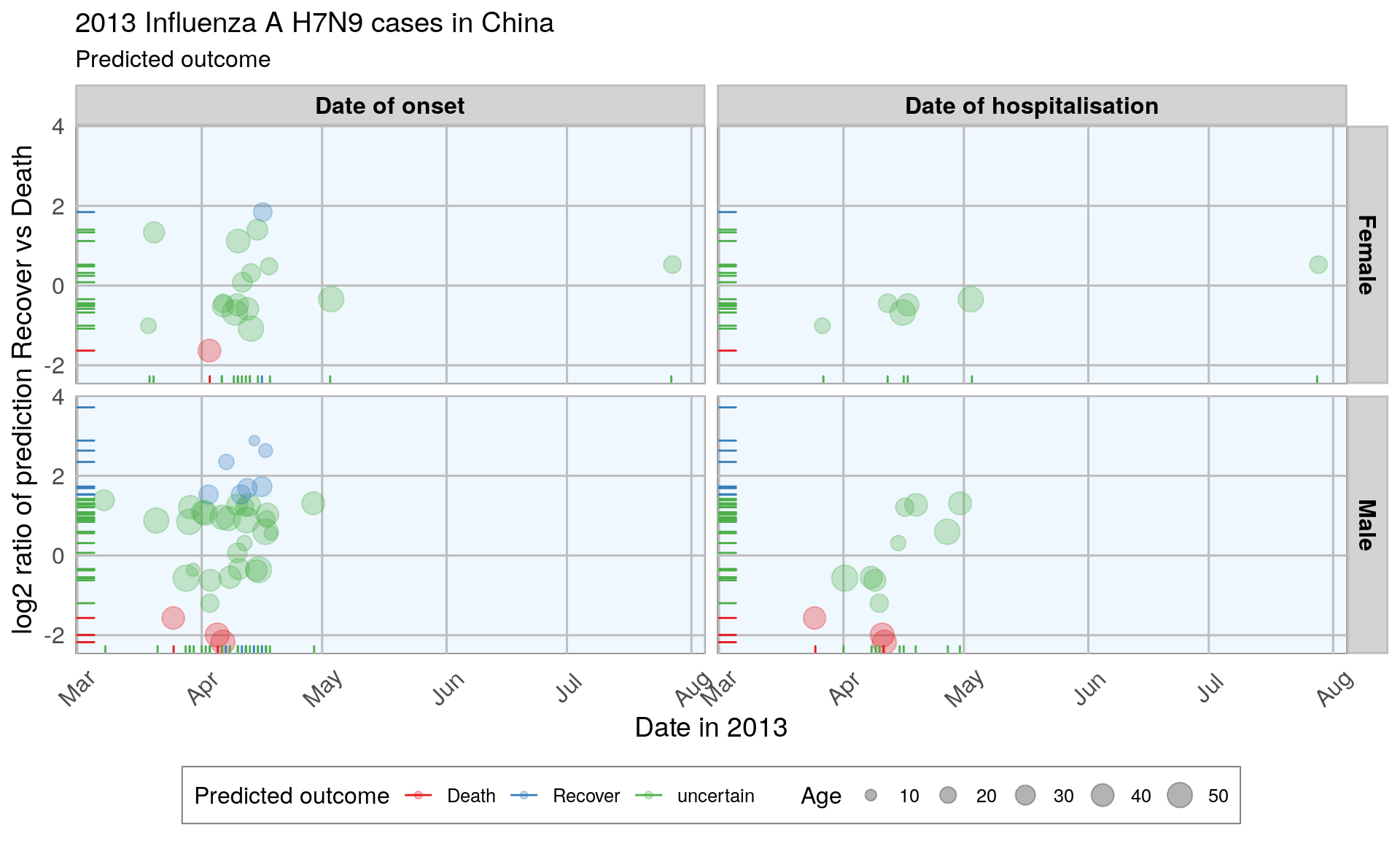
The comparison of date of onset, data of hospitalization, gender and age with predicted outcome shows that predicted deaths were associated with older age than predicted recoveries. Date of onset does not show an obvious bias in either direction.
28.8 Conclusions
This dataset posed a couple of difficulties to begin with, like unequal distribution of data points across variables and missing data. This makes the modeling inherently prone to flaws. However, real life data isn’t perfect either, so I went ahead and tested the modeling success anyway.
By accounting for uncertain classification with low predictions probability, the validation data could be classified accurately. However, for a more accurate model, these few cases don’t give enough information to reliably predict the outcome. More cases, more information (i.e. more features) and fewer missing data would improve the modeling outcome.
Also, this example is only applicable for this specific case of flu. In order to be able to draw more general conclusions about flu outcome, other cases and additional information, for example on medical parameters like preexisting medical conditions, disase parameters, demographic information, etc. would be necessary.
All in all, this dataset served as a nice example of the possibilities (and pitfalls) of machine learning applications and showcases a basic workflow for building prediction models with R.
For a comparison of feature selection methods see here.
If you see any mistakes or have tips and tricks for improvement, please don’t hesitate to let me know! Thanks. :-)
sessionInfo()
#> R version 3.6.3 (2020-02-29)
#> Platform: x86_64-pc-linux-gnu (64-bit)
#> Running under: Debian GNU/Linux 10 (buster)
#>
#> Matrix products: default
#> BLAS/LAPACK: /usr/lib/x86_64-linux-gnu/libopenblasp-r0.3.5.so
#>
#> locale:
#>  [1] LC_CTYPE=en_US.UTF-8       LC_NUMERIC=C               LC_TIME=en_US.UTF-8        LC_COLLATE=en_US.UTF-8     LC_MONETARY=en_US.UTF-8    LC_MESSAGES=C              LC_PAPER=en_US.UTF-8       LC_NAME=C                  LC_ADDRESS=C               LC_TELEPHONE=C             LC_MEASUREMENT=en_US.UTF-8 LC_IDENTIFICATION=C
#>
#> attached base packages:
#> [1] grid      stats     graphics  grDevices utils     datasets  methods   base
#>
#> other attached packages:
#>  [1] RColorBrewer_1.1-2 rpart.plot_3.0.8   rattle_5.3.0       rpart_4.1-15       caret_6.0-86       lattice_0.20-38    mice_3.8.0         dplyr_0.8.5        gridExtra_2.3      ggplot2_3.3.0      plyr_1.8.6         tidyr_1.0.2        outbreaks_1.5.0
#>
#> loaded via a namespace (and not attached):
#>  [1] nlme_3.1-144         fs_1.4.1             lubridate_1.7.8      C50_0.1.3            tools_3.6.3          backports_1.1.6      bslib_0.2.2.9000     utf8_1.1.4           R6_2.4.1             colorspace_1.4-1     nnet_7.3-12          withr_2.2.0          tidyselect_1.0.0     downlit_0.2.1.9000   compiler_3.6.3       mda_0.4-10           cli_2.0.2            glmnet_3.0-2         xml2_1.3.2           isoband_0.2.1        Cubist_0.2.3         labeling_0.3         bookdown_0.21.4      sass_0.2.0.9005      scales_1.1.0         mvtnorm_1.1-0        randomForest_4.6-14  rappdirs_0.3.1       stringr_1.4.0        digest_0.6.25        rmarkdown_2.5.3      pkgconfig_2.0.3      htmltools_0.5.0.9003 rlang_0.4.5          shape_1.4.4          jquerylib_0.1.2      farver_2.0.3         generics_0.0.2       jsonlite_1.6.1       ModelMetrics_1.2.2.2 magrittr_1.5         Formula_1.2-3        Matrix_1.2-18        fansi_0.4.1          Rcpp_1.0.4.6         munsell_0.5.0        partykit_1.2-7
#> [48] lifecycle_0.2.0      stringi_1.4.6        pROC_1.16.2          yaml_2.2.1           inum_1.0-1           MASS_7.3-51.5        pamr_1.56.1          recipes_0.1.10       pls_2.7-2            crayon_1.3.4         splines_3.6.3        knitr_1.28           pillar_1.4.3         igraph_1.2.5         reshape2_1.4.4       codetools_0.2-16     stats4_3.6.3         glue_1.4.0           evaluate_0.14        data.table_1.12.8    vctrs_0.2.4          foreach_1.5.0        gtable_0.3.0         purrr_0.3.4          assertthat_0.2.1     xfun_0.19.4          gower_0.2.1          prodlim_2019.11.13   libcoin_1.0-5        broom_0.5.6          e1071_1.7-3          class_7.3-15         survival_3.1-8       timeDate_3043.102    tibble_3.0.1         iterators_1.0.12     kknn_1.3.1           cluster_2.1.0        lava_1.6.7           ellipsis_0.3.0       ipred_0.9-9