36 Regression with a neural network
- Dataset:
BostonHousing - Algorithms:
- Neural Network (
nnet) - Linear Regression
- Neural Network (
###
### prepare data
###
library(mlbench)
data(BostonHousing)

# inspect the range which is 1-50
summary(BostonHousing$medv)
#>    Min. 1st Qu.  Median    Mean 3rd Qu.    Max.
#>     5.0    17.0    21.2    22.5    25.0    50.0


##
## model linear regression
##

lm.fit <- lm(medv ~ ., data=BostonHousing)

lm.predict <- predict(lm.fit)

# mean squared error: 21.89483
mean((lm.predict - BostonHousing$medv)^2)
#> [1] 21.9

plot(BostonHousing$medv, lm.predict,
    main="Linear regression predictions vs actual",
    xlab="Actual")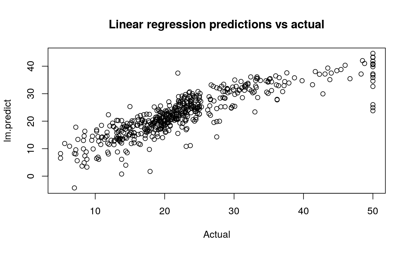
##
## model neural network
##
require(nnet)
#> Loading required package: nnet

# scale inputs: divide by 50 to get 0-1 range
nnet.fit <- nnet(medv/50 ~ ., data=BostonHousing, size=2)
#> # weights:  31
#> initial  value 17.039194
#> iter  10 value 13.754559
#> iter  20 value 13.537235
#> iter  30 value 13.537183
#> iter  40 value 13.530522
#> final  value 13.529736
#> converged

# multiply 50 to restore original scale
nnet.predict <- predict(nnet.fit)*50

# mean squared error: 16.40581
mean((nnet.predict - BostonHousing$medv)^2)
#> [1] 66.8

plot(BostonHousing$medv, nnet.predict,
    main="Neural network predictions vs actual",
    xlab="Actual")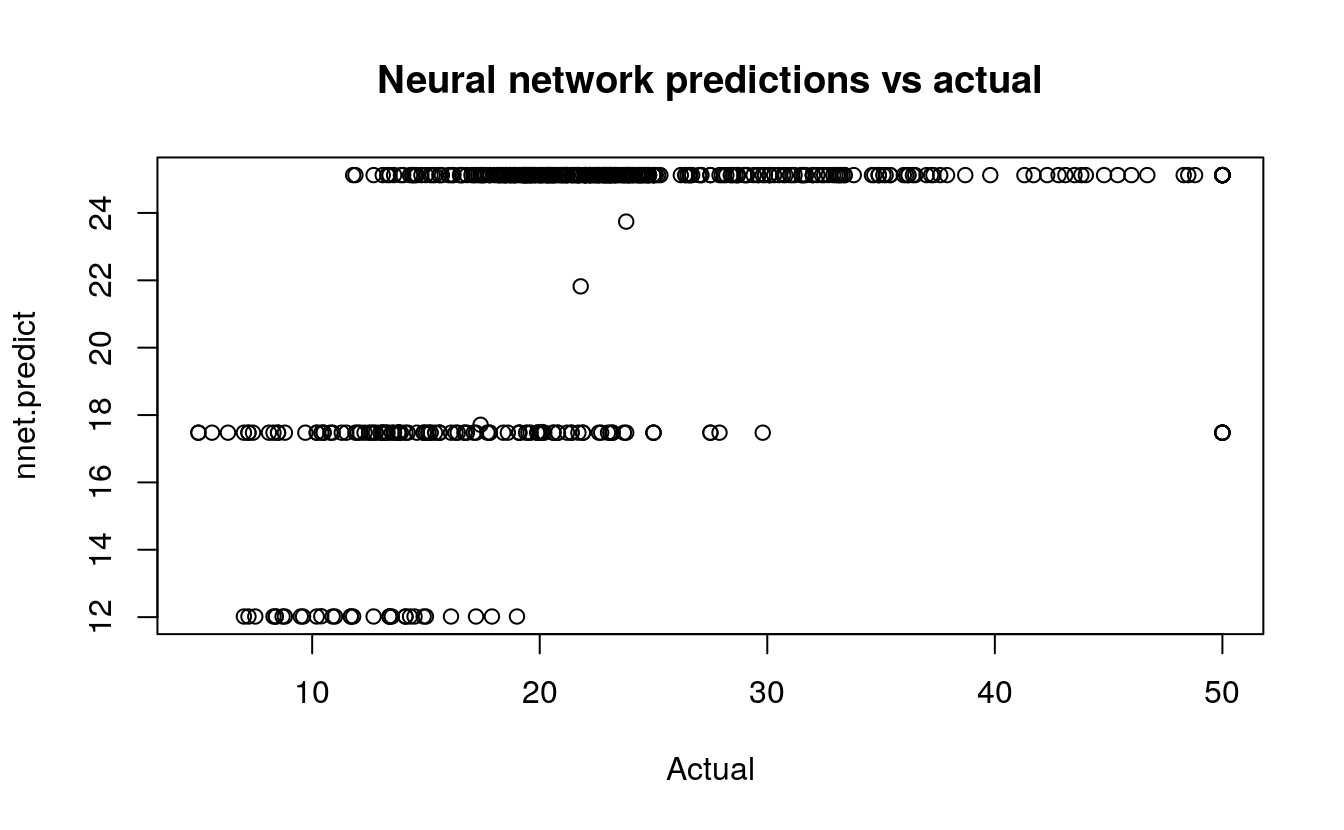
36.1 Neural Network
Now, let’s use the function train() from the package caret to optimize the neural network hyperparameters decay and size, Also, caret performs resampling to give a better estimate of the error. In this case we scale linear regression by the same value, so the error statistics are directly comparable.
 library(mlbench)
 data(BostonHousing)

require(caret)
#> Loading required package: caret
#> Loading required package: lattice
#> Loading required package: ggplot2

mygrid <- expand.grid(.decay=c(0.5, 0.1), .size=c(4,5,6))
nnetfit <- train(medv/50 ~ ., data=BostonHousing, method="nnet", maxit=1000, tuneGrid=mygrid, trace=F)
print(nnetfit)
#> Neural Network
#>
#> 506 samples
#>  13 predictor
#>
#> No pre-processing
#> Resampling: Bootstrapped (25 reps)
#> Summary of sample sizes: 506, 506, 506, 506, 506, 506, ...
#> Resampling results across tuning parameters:
#>
#>   decay  size  RMSE    Rsquared  MAE
#>   0.1    4     0.0830  0.790     0.0571
#>   0.1    5     0.0814  0.798     0.0559
#>   0.1    6     0.0799  0.806     0.0549
#>   0.5    4     0.0908  0.757     0.0626
#>   0.5    5     0.0897  0.762     0.0622
#>   0.5    6     0.0890  0.766     0.0620
#>
#> RMSE was used to select the optimal model using the smallest value.
#> The final values used for the model were size = 6 and decay = 0.1.
506 samples
13 predictors
No pre-processing
Resampling: Bootstrap (25 reps)
Summary of sample sizes: 506, 506, 506, 506, 506, 506, ...
Resampling results across tuning parameters:
size decay RMSE Rsquared RMSE SD Rsquared SD
4 0.1 0.0852 0.785 0.00863 0.0406
4 0.5 0.0923 0.753 0.00891 0.0436
5 0.1 0.0836 0.792 0.00829 0.0396
5 0.5 0.0899 0.765 0.00858 0.0399
6 0.1 0.0835 0.793 0.00804 0.0318
6 0.5 0.0895 0.768 0.00789 0.0344 36.2 Linear Regression
 lmfit <- train(medv/50 ~ ., data=BostonHousing, method="lm")
 print(lmfit)
#> Linear Regression
#>
#> 506 samples
#>  13 predictor
#>
#> No pre-processing
#> Resampling: Bootstrapped (25 reps)
#> Summary of sample sizes: 506, 506, 506, 506, 506, 506, ...
#> Resampling results:
#>
#>   RMSE    Rsquared  MAE
#>   0.0988  0.726     0.0692
#>
#> Tuning parameter 'intercept' was held constant at a value of TRUE
506 samples
13 predictors
No pre-processing
Resampling: Bootstrap (25 reps)
Summary of sample sizes: 506, 506, 506, 506, 506, 506, ...
Resampling results
RMSE Rsquared RMSE SD Rsquared SD
0.0994 0.703 0.00741 0.0389 A tuned neural network has a RMSE of 0.0835 compared to linear regression’s RMSE of 0.0994.