6.1 Introduction

https://beckmw.wordpress.com/tag/nnet/

I’ve made quite a few blog posts about neural networks and some of the diagnostic tools that can be used to ‘demystify’ the information contained in these models. Frankly, I’m kind of sick of writing about neural networks but I wanted to share one last tool I’ve implemented in R. I’m a strong believer that supervised neural networks can be used for much more than prediction, as is the common assumption by most researchers. I hope that my collection of posts, including this one, has shown the versatility of these models to develop inference into causation. To date, I’ve authored posts on visualizing neural networks, animating neural networks, and determining importance of model inputs. This post will describe a function for a sensitivity analysis of a neural network. Specifically, I will describe an approach to evaluate the form of the relationship of a response variable with the explanatory variables used in the model.

The general goal of a sensitivity analysis is similar to evaluating relative importance of explanatory variables, with a few important distinctions. For both analyses, we are interested in the relationships between explanatory and response variables as described by the model in the hope that the neural network has explained some real-world phenomenon. Using Garson’s algorithm,1 we can get an idea of the magnitude and sign of the relationship between variables relative to each other. Conversely, the sensitivity analysis allows us to obtain information about the form of the relationship between variables rather than a categorical description, such as variable x is positively and strongly related to y. For example, how does a response variable change in relation to increasing or decreasing values of a given explanatory variable? Is it a linear response, non-linear, uni-modal, no response, etc.? Furthermore, how does the form of the response change given values of the other explanatory variables in the model? We might expect that the relationship between a response and explanatory variable might differ given the context of the other explanatory variables (i.e., an interaction may be present). The sensitivity analysis can provide this information.

As with most of my posts, I’ve created the sensitivity analysis function using ideas from other people that are much more clever than me. I’ve simply converted these ideas into a useful form in R. Ultimate credit for the sensitivity analysis goes to Sovan Lek (and colleagues), who developed the approach in the mid-1990s. The ‘Lek-profile method’ is described briefly in Lek et al. 19962 and in more detail in Gevrey et al. 2003.3 I’ll provide a brief summary here since the method is pretty simple. In fact, the profile method can be extended to any statistical model and is not specific to neural networks, although it is one of few methods used to evaluate the latter. For any statistical model where multiple response variables are related to multiple explanatory variables, we choose one response and one explanatory variable. We obtain predictions of the response variable across the range of values for the given explanatory variable. All other explanatory variables are held constant at a given set of respective values (e.g., minimum, 20th percentile, maximum). The final product is a set of response curves for one response variable across the range of values for one explanatory variable, while holding all other explanatory variables constant. This is implemented in R by creating a matrix of values for explanatory variables where the number of rows is the number of observations and the number of columns is the number of explanatory variables. All explanatory variables are held at their mean (or other constant value) while the variable of interest is sequenced from its minimum to maximum value across the range of observations. This matrix (actually a data frame) is then used to predict values of the response variable from a fitted model object. This is repeated for different variables.

I’ll illustrate the function using simulated data, as I’ve done in previous posts. The exception here is that I’ll be using two response variables instead of one. The two response variables are linear combinations of eight explanatory variables, with random error components taken from a normal distribution. The relationships between the variables are determined by the arbitrary set of parameters (parms1 and parms2). The explanatory variables are partially correlated and taken from a multivariate normal distribution.

require(clusterGeneration)
#> Loading required package: clusterGeneration
#> Loading required package: MASS
require(nnet)
#> Loading required package: nnet
  
#define number of variables and observations
set.seed(2)
num.vars<-8
num.obs<-10000
  
#define correlation matrix for explanatory variables 
#define actual parameter values
cov.mat<-genPositiveDefMat(num.vars,covMethod=c("unifcorrmat"))$Sigma
rand.vars<-mvrnorm(num.obs,rep(0,num.vars),Sigma=cov.mat)
parms1<-runif(num.vars,-10,10)
y1<-rand.vars %*% matrix(parms1) + rnorm(num.obs,sd=20)
parms2<-runif(num.vars,-10,10)
y2<-rand.vars %*% matrix(parms2) + rnorm(num.obs,sd=20)
 
#prep data and create neural network
rand.vars<-data.frame(rand.vars)
resp<-apply(cbind(y1,y2),2, function(y) (y-min(y))/(max(y)-min(y)))
resp<-data.frame(resp)
names(resp)<-c('Y1','Y2')

mod1 <- nnet(rand.vars,resp,size=8,linout=T)
#> # weights:  90
#> initial  value 30121.205794 
#> iter  10 value 130.537462
#> iter  20 value 57.187090
#> iter  30 value 47.285919
#> iter  40 value 42.778564
#> iter  50 value 39.837784
#> iter  60 value 36.694632
#> iter  70 value 35.140948
#> iter  80 value 34.268819
#> iter  90 value 33.772282
#> iter 100 value 33.472654
#> final  value 33.472654 
#> stopped after 100 iterations

#import the function from Github
library(devtools)
#> Loading required package: usethis

# source_url('https://gist.githubusercontent.com/fawda123/7471137/raw/466c1474d0a505ff044412703516c34f1a4684a5/nnet_plot_update.r')
source("nnet_plot_update.r")
 
#plot each model
plot.nnet(mod1)
#> Loading required package: scales
#> Loading required package: reshape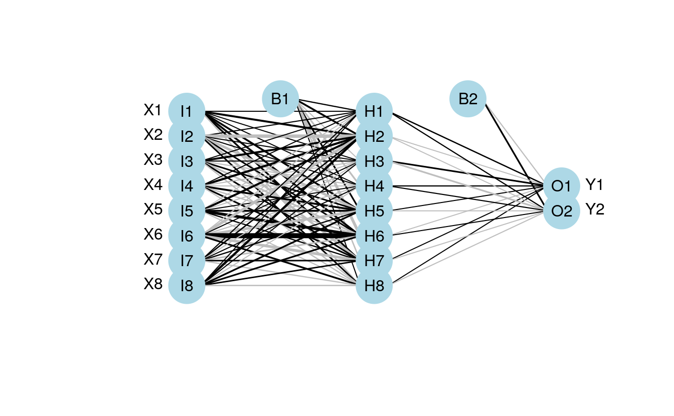

6.2 The Lek profile function

We’ve created a neural network that hopefully describes the relationship of two response variables with eight explanatory variables. The sensitivity analysis lets us visualize these relationships. The Lek profile function can be used once we have a neural network model in our workspace. The function is imported and used as follows:

# source('https://gist.githubusercontent.com/fawda123/6860630/raw/b8bf4a6c88d6b392b1bfa6ef24759ae98f31877c/lek_fun.r')
source("lek_fun.r")

lek.fun(mod1)
#> Loading required package: ggplot2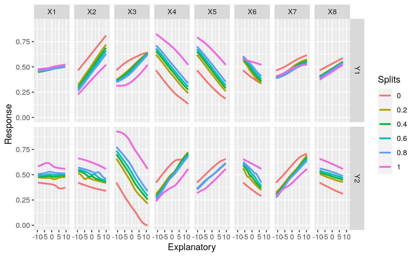

Fig: Sensitivity analysis of the two response variables in the neural network model to individual explanatory variables. Splits represent the quantile values at which the remaining explanatory variables were held constant. The function can be obtained here

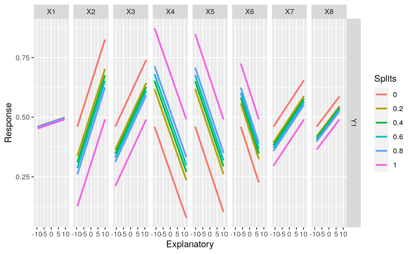
By default, the function runs a sensitivity analysis for all variables. This creates a busy plot so we may want to look at specific variables of interest. Maybe we want to evaluate different quantile values as well. These options can be changed using the arguments.

lek.fun(mod1,var.sens=c('X2','X5'),split.vals=seq(0,1,by=0.05))

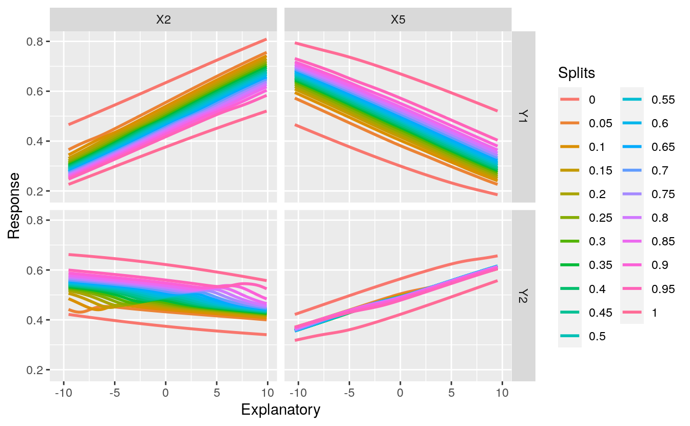
Fig: Sensitivity analysis of the two response variables in relation to explanatory variables X2 and X5 and different quantile values for the remaining variables.

The function also returns a ggplot2 object that can be further modified. You may prefer a different theme, color, or line type, for example.

p1<-lek.fun(mod1)
class(p1)
#> [1] "gg"     "ggplot"
# [1] "gg"     "ggplot"
 
p1 + 
   theme_bw() +
   scale_colour_brewer(palette="PuBu") +
   scale_linetype_manual(values=rep('dashed',6)) +
   scale_size_manual(values=rep(1,6))
#> Scale for 'linetype' is already present. Adding another scale for 'linetype',
#> which will replace the existing scale.
#> Scale for 'size' is already present. Adding another scale for 'size', which
#> will replace the existing scale.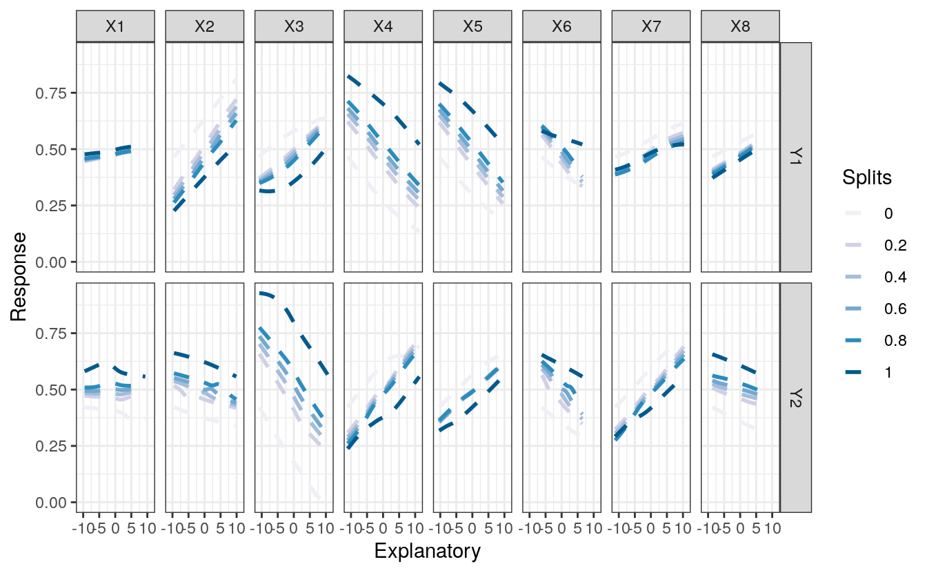

6.3 Getting a dataframe from lek

Finally, the actual values from the sensitivity analysis can be returned if you’d prefer that instead. The output is a data frame in long form that was created using melt.list from the reshape package for compatibility with ggplot2. The six columns indicate values for explanatory variables on the x-axes, names of the response variables, predicted values of the response variables, quantiles at which other explanatory variables were held constant, and names of the explanatory variables on the x-axes.

head(lek.fun(mod1,val.out = TRUE))
#>   Explanatory resp.name Response Splits exp.name
#> 1       -9.58        Y1    0.466      0       X1
#> 2       -9.39        Y1    0.466      0       X1
#> 3       -9.19        Y1    0.467      0       X1
#> 4       -9.00        Y1    0.467      0       X1
#> 5       -8.81        Y1    0.468      0       X1
#> 6       -8.62        Y1    0.468      0       X1

6.4 The lek function works with lm

I mentioned earlier that the function is not unique to neural networks and can work with other models created in R. I haven’t done an extensive test of the function, but I’m fairly certain that it will work if the model object has a predict method (e.g., predict.lm). Here’s an example using the function to evaluate a multiple linear regression for one of the response variables.

mod2 <-lm(Y1 ~ ., data = cbind(resp[,'Y1', drop = F], rand.vars))
lek.fun(mod2)

This function has little relevance for conventional models like linear regression since a wealth of diagnostic tools are already available (e.g., effects plots, add/drop procedures, outlier tests, etc.). The application of the function to neural networks provides insight into the relationships described by the models, insights that to my knowledge, cannot be obtained using current tools in R. This post concludes my contribution of diagnostic tools for neural networks in R and I hope that they have been useful to some of you. I have spent the last year or so working with neural networks and my opinion of their utility is mixed. I see advantages in the use of highly flexible computer-based algorithms, although in most cases similar conclusions can be made using more conventional analyses. I suggest that neural networks only be used if there is an extremely high sample size and other methods have proven inconclusive. Feel free to voice your opinions or suggestions in the comments.

6.5 lek function works with RSNNS

require(clusterGeneration)
require(RSNNS)
#> Loading required package: RSNNS
#> Loading required package: Rcpp
require(devtools)
 
#define number of variables and observations
set.seed(2)
num.vars<-8
num.obs<-10000
 
#define correlation matrix for explanatory variables 
#define actual parameter values
cov.mat <-genPositiveDefMat(num.vars,covMethod=c("unifcorrmat"))$Sigma
rand.vars <-mvrnorm(num.obs,rep(0,num.vars),Sigma=cov.mat)
parms1 <-runif(num.vars,-10,10)
y1 <-rand.vars %*% matrix(parms1) + rnorm(num.obs,sd=20)
parms2 <-runif(num.vars,-10,10)
y2 <-rand.vars %*% matrix(parms2) + rnorm(num.obs,sd=20)
 
#prep data and create neural network
rand.vars <- data.frame(rand.vars)
resp <- apply(cbind(y1,y2),2, function(y) (y-min(y))/(max(y)-min(y)))
resp <- data.frame(resp)
names(resp)<-c('Y1','Y2')

tibble::as_tibble(rand.vars)
#> # A tibble: 10,000 x 8
#>        X1     X2     X3     X4     X5    X6    X7     X8
#>     <dbl>  <dbl>  <dbl>  <dbl>  <dbl> <dbl> <dbl>  <dbl>
#> 1  1.61    2.13   2.13   3.97  -1.34   2.00  3.11 -2.55 
#> 2 -1.25    3.07  -0.325  1.61  -0.484  2.28  2.98 -1.71 
#> 3 -3.17   -1.29  -1.77  -1.66  -0.549 -3.19  1.07  1.81 
#> 4 -2.39    3.28  -3.42  -0.160 -1.52   2.67  7.05 -1.14 
#> 5 -1.55   -0.181 -1.14   2.27  -1.68  -1.67  3.08  0.334
#> 6  0.0690 -1.54  -2.98   2.84   1.42   1.31  1.82  2.07 
#> # … with 9,994 more rows

tibble::as_tibble(resp)
#> # A tibble: 10,000 x 2
#>      Y1    Y2
#>   <dbl> <dbl>
#> 1 0.461 0.500
#> 2 0.416 0.509
#> 3 0.534 0.675
#> 4 0.548 0.619
#> 5 0.519 0.659
#> 6 0.389 0.622
#> # … with 9,994 more rows

# create neural network model
mod2 <- mlp(rand.vars, resp, size = 8, linOut = T)
 
#import sensitivity analysis function
source_url('https://gist.githubusercontent.com/fawda123/6860630/raw/b8bf4a6c88d6b392b1bfa6ef24759ae98f31877c/lek_fun.r')
#> SHA-1 hash of file is 4a2d33b94a08f46a94518207a4ae7cc412845222
 
#sensitivity analsyis, note 'exp.in' argument
lek.fun(mod2, exp.in = rand.vars)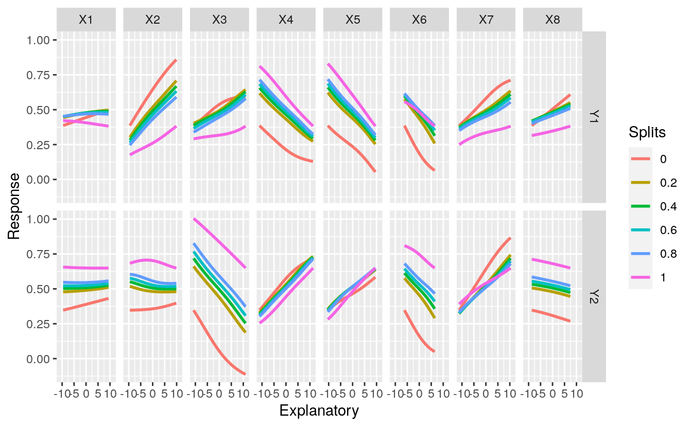

6.6 References

1 Garson GD. 1991. Interpreting neural network connection weights. Artificial Intelligence Expert. 6:46–51. 2 Lek S, Delacoste M, Baran P, Dimopoulos I, Lauga J, Aulagnier S. 1996. Application of neural networks to modelling nonlinear relationships in Ecology. Ecological Modelling. 90:39-52. 3 Gevrey M, Dimopoulos I, Lek S. 2003. Review and comparison of methods to study the contribution of variables in artificial neural network models. Ecological Modelling. 160:249-264.