14 Imputting missing values with Random Forest
14.1 Flu Prediction. fluH7N9_china_2013 dataset
Source: https://shirinsplayground.netlify.com/2018/04/flu_prediction/
library(outbreaks)
library(tidyverse)
library(plyr)
library(mice)
library(caret)
library(purrr)
library("tibble")
library("dplyr")
library("tidyr")
Since I migrated my blog from Github Pages to blogdown and Netlify, I wanted to start migrating (most of) my old posts too - and use that opportunity to update them and make sure the code still works.
Here I am updating my very first machine learning post from 27 Nov 2016: Can we predict flu deaths with Machine Learning and R?. Changes are marked as bold comments.
The main changes I made are:
using the tidyverse more consistently throughout the analysis
focusing on comparing multiple imputations from the mice package, rather than comparing different algorithms
using purrr, map(), nest() and unnest() to model and predict the machine learning algorithm over the different imputed datasets
Among the many nice R packages containing data collections is the outbreaks package. It contains a dataset on epidemics and among them is data from the 2013 outbreak of influenza A H7N9 in China as analysed by Kucharski et al. (2014):
A. Kucharski, H. Mills, A. Pinsent, C. Fraser, M. Van Kerkhove, C. A. Donnelly, and S. Riley. 2014. Distinguishing between reservoir exposure and human-to-human transmission for emerging pathogens using case onset data. PLOS Currents Outbreaks. Mar 7, edition 1. doi: 10.1371/currents.outbreaks.e1473d9bfc99d080ca242139a06c455f.
A. Kucharski, H. Mills, A. Pinsent, C. Fraser, M. Van Kerkhove, C. A. Donnelly, and S. Riley. 2014. Data from: Distinguishing between reservoir exposure and human-to-human transmission for emerging pathogens using case onset data. Dryad Digital Repository. http://dx.doi.org/10.5061/dryad.2g43n.
I will be using their data as an example to show how to use Machine Learning algorithms for predicting disease outcome.
14.2 The data
The dataset contains case ID, date of onset, date of hospitalization, date of outcome, gender, age, province and of course outcome: Death or Recovery.
14.2.1 Pre-processing
Change: variable names (i.e. column names) have been renamed, dots have been replaced with underscores, letters are all lower case now.
Change: I am using the tidyverse notation more consistently.
First, I’m doing some preprocessing, including:
- renaming missing data as NA
- adding an ID column
- setting column types
- gathering date columns
- changing factor names of dates (to make them look nicer in plots) and of province (to combine provinces with few cases)
from1 <- c("date_of_onset", "date_of_hospitalisation", "date_of_outcome")
to1   <- c("date of onset", "date of hospitalisation", "date of outcome")
from2 <- c("Anhui", "Beijing", "Fujian", "Guangdong", "Hebei", "Henan",
           "Hunan", "Jiangxi", "Shandong", "Taiwan")
to2   <- rep("Other", 10)

fluH7N9_china_2013$age[which(fluH7N9_china_2013$age == "?")] <- NA
fluH7N9_china_2013_gather <- fluH7N9_china_2013 %>%
  mutate(case_id = paste("case", case_id, sep = "_"),
         age = as.numeric(age)) %>%
  gather(Group, Date, date_of_onset:date_of_outcome) %>%
  mutate(Group = as.factor(mapvalues(Group, from = from1, to = to1)),
         province = mapvalues(province, from = from2, to = to2))

fluH7N9_china_2013 <- as.tibble(fluH7N9_china_2013)
#> Warning: `as.tibble()` is deprecated as of tibble 2.0.0.
#> Please use `as_tibble()` instead.
#> The signature and semantics have changed, see `?as_tibble`.
#> This warning is displayed once every 8 hours.
#> Call `lifecycle::last_warnings()` to see where this warning was generated.
fluH7N9_china_2013_gather <- as.tibble(fluH7N9_china_2013_gather)
print(fluH7N9_china_2013)
#> # A tibble: 136 x 8
#>   case_id date_of_onset date_of_hospita… date_of_outcome outcome gender age
#>   <fct>   <date>        <date>           <date>          <fct>   <fct>  <fct>
#> 1 1       2013-02-19    NA               2013-03-04      Death   m      87
#> 2 2       2013-02-27    2013-03-03       2013-03-10      Death   m      27
#> 3 3       2013-03-09    2013-03-19       2013-04-09      Death   f      35
#> 4 4       2013-03-19    2013-03-27       NA              <NA>    f      45
#> 5 5       2013-03-19    2013-03-30       2013-05-15      Recover f      48
#> 6 6       2013-03-21    2013-03-28       2013-04-26      Death   f      32
#> # … with 130 more rows, and 1 more variable: province <fct>
I’m also adding a third gender level for unknown gender
levels(fluH7N9_china_2013_gather$gender) <-
  c(levels(fluH7N9_china_2013_gather$gender), "unknown")
fluH7N9_china_2013_gather$gender[is.na(fluH7N9_china_2013_gather$gender)] <- "unknown"
print(fluH7N9_china_2013_gather)
#> # A tibble: 408 x 7
#>   case_id outcome gender   age province Group         Date
#>   <chr>   <fct>   <fct>  <dbl> <fct>    <fct>         <date>
#> 1 case_1  Death   m         58 Shanghai date of onset 2013-02-19
#> 2 case_2  Death   m          7 Shanghai date of onset 2013-02-27
#> 3 case_3  Death   f         11 Other    date of onset 2013-03-09
#> 4 case_4  <NA>    f         18 Jiangsu  date of onset 2013-03-19
#> 5 case_5  Recover f         20 Jiangsu  date of onset 2013-03-19
#> 6 case_6  Death   f          9 Jiangsu  date of onset 2013-03-21
#> # … with 402 more rows
For plotting, I am defining a custom ggplot2 theme:
my_theme <- function(base_size = 12, base_family = "sans"){
  theme_minimal(base_size = base_size, base_family = base_family) +
  theme(
    axis.text = element_text(size = 12),
    axis.text.x = element_text(angle = 45, vjust = 0.5, hjust = 0.5),
    axis.title = element_text(size = 14),
    panel.grid.major = element_line(color = "grey"),
    panel.grid.minor = element_blank(),
    panel.background = element_rect(fill = "aliceblue"),
    strip.background = element_rect(fill = "lightgrey", color = "grey", size = 1),
    strip.text = element_text(face = "bold", size = 12, color = "black"),
    legend.position = "bottom",
    legend.justification = "top",
    legend.box = "horizontal",
    legend.box.background = element_rect(colour = "grey50"),
    legend.background = element_blank(),
    panel.border = element_rect(color = "grey", fill = NA, size = 0.5)
  )
}
And use that theme to visualize the data:
ggplot(data = fluH7N9_china_2013_gather, aes(x = Date, y = age, fill = outcome)) +
  stat_density2d(aes(alpha = ..level..), geom = "polygon") +
  geom_jitter(aes(color = outcome, shape = gender), size = 1.5) +
  geom_rug(aes(color = outcome)) +
  scale_y_continuous(limits = c(0, 90)) +
  labs(
    fill = "Outcome",
    color = "Outcome",
    alpha = "Level",
    shape = "Gender",
    x = "Date in 2013",
    y = "Age",
    title = "2013 Influenza A H7N9 cases in China",
    subtitle = "Dataset from 'outbreaks' package (Kucharski et al. 2014)",
    caption = ""
  ) +
  facet_grid(Group ~ province) +
  my_theme() +
  scale_shape_manual(values = c(15, 16, 17)) +
  scale_color_brewer(palette="Set1", na.value = "grey50") +
  scale_fill_brewer(palette="Set1")
#> Warning: Removed 149 rows containing non-finite values (stat_density2d).
#> Warning: Removed 149 rows containing missing values (geom_point).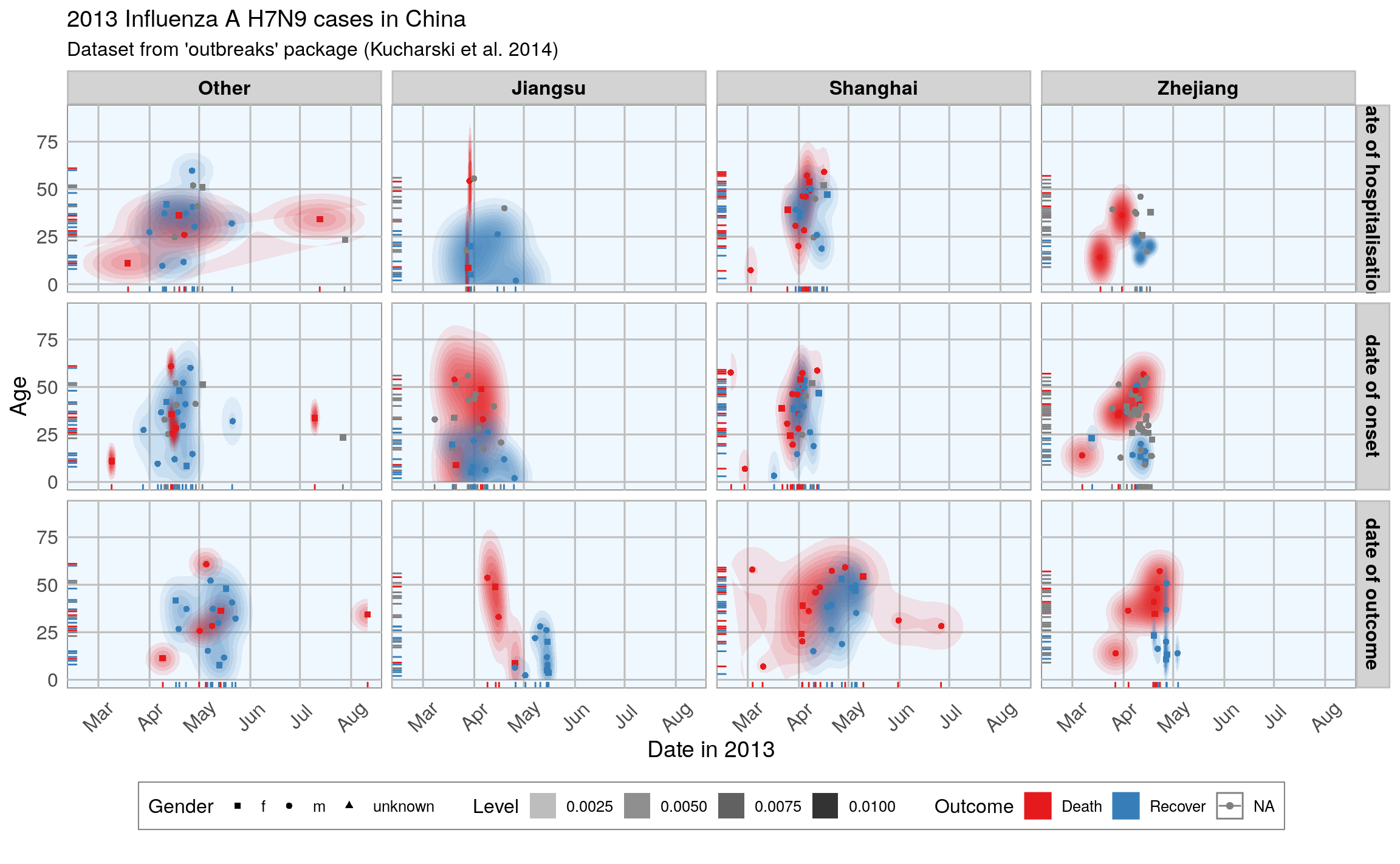
ggplot(data = fluH7N9_china_2013_gather, aes(x = Date, y = age, color = outcome)) +
  geom_point(aes(color = outcome, shape = gender), size = 1.5, alpha = 0.6) +
  geom_path(aes(group = case_id)) +
  facet_wrap( ~ province, ncol = 2) +
  my_theme() +
  scale_shape_manual(values = c(15, 16, 17)) +
  scale_color_brewer(palette="Set1", na.value = "grey50") +
  scale_fill_brewer(palette="Set1") +
  labs(
    color = "Outcome",
    shape = "Gender",
    x = "Date in 2013",
    y = "Age",
    title = "2013 Influenza A H7N9 cases in China",
    subtitle = "Dataset from 'outbreaks' package (Kucharski et al. 2014)",
    caption = "\nTime from onset of flu to outcome."
  )
#> Warning: Removed 149 rows containing missing values (geom_point).
#> Warning: Removed 122 row(s) containing missing values (geom_path).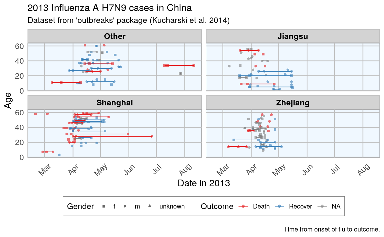
14.3 Features
In machine learning-speak features are what we call the variables used for model training. Using the right features dramatically influences the accuracy and success of your model.
For this example, I am keeping age, but I am also generating new features from the date information and converting gender and province into numerical values.
delta_dates <- function(onset, ref) {
    d2 = as.Date(as.character(onset), format = "%Y-%m-%d")
    d1 = as.Date(as.character(ref), format = "%Y-%m-%d")
    as.numeric(as.character(gsub(" days", "", d1 - d2)))
}
dataset <- fluH7N9_china_2013 %>%
  mutate(
      hospital = as.factor(ifelse(is.na(date_of_hospitalisation), 0, 1)),
      gender_f = as.factor(ifelse(gender == "f", 1, 0)),
      province_Jiangsu = as.factor(ifelse(province == "Jiangsu", 1, 0)),
      province_Shanghai = as.factor(ifelse(province == "Shanghai", 1, 0)),
      province_Zhejiang = as.factor(ifelse(province == "Zhejiang", 1, 0)),
      province_other = as.factor(ifelse(province == "Zhejiang"
                                           | province == "Jiangsu"
                                           | province == "Shanghai", 0, 1)),

      days_onset_to_outcome = delta_dates(date_of_onset, date_of_outcome),
      days_onset_to_hospital = delta_dates(date_of_onset, date_of_hospitalisation),
      age = age,
      early_onset = as.factor(ifelse(date_of_onset <
                                     summary(date_of_onset)[[3]], 1, 0)),
      early_outcome = as.factor(ifelse(date_of_outcome <
                                       summary(date_of_outcome)[[3]], 1, 0))
    ) %>%
  subset(select = -c(2:4, 6, 8))
# convert tibble to data.frame; tibble causing error
dataset_df <- as.data.frame(dataset)
rownames(dataset_df) <- dataset_df$case_id
dataset_df[, -2] <- as.numeric(as.matrix(dataset_df[, -2]))
dataset <- dataset_df     # copy to dataset object
glimpse(dataset)
#> Rows: 136
#> Columns: 13
#> $ case_id                <dbl> 1, 2, 3, 4, 5, 6, 7, 8, 9, 10, 11, 12, 13, 14,…
#> $ outcome                <fct> Death, Death, Death, NA, Recover, Death, Death…
#> $ age                    <dbl> 87, 27, 35, 45, 48, 32, 83, 38, 67, 48, 64, 52…
#> $ hospital               <dbl> 0, 1, 1, 1, 1, 1, 1, 1, 1, 1, 1, 0, 1, 0, 0, 0…
#> $ gender_f               <dbl> 0, 0, 1, 1, 1, 1, 0, 0, 0, 0, 0, 1, 1, 0, 1, 0…
#> $ province_Jiangsu       <dbl> 0, 0, 0, 1, 1, 1, 1, 0, 0, 0, 0, 0, 0, 0, 1, 1…
#> $ province_Shanghai      <dbl> 1, 1, 0, 0, 0, 0, 0, 0, 0, 1, 0, 1, 1, 1, 0, 0…
#> $ province_Zhejiang      <dbl> 0, 0, 0, 0, 0, 0, 0, 1, 1, 0, 1, 0, 0, 0, 0, 0…
#> $ province_other         <dbl> 0, 0, 1, 0, 0, 0, 0, 0, 0, 0, 0, 0, 0, 0, 0, 0…
#> $ days_onset_to_outcome  <dbl> 13, 11, 31, NA, 57, 36, 20, 20, NA, 6, 6, 7, 1…
#> $ days_onset_to_hospital <dbl> NA, 4, 10, 8, 11, 7, 9, 11, 0, 4, 2, NA, 3, NA…
#> $ early_onset            <dbl> 1, 1, 1, 1, 1, 1, 1, 1, 1, 1, 1, 1, 1, 1, 1, 1…
#> $ early_outcome          <dbl> 1, 1, 1, NA, 0, 1, 1, 1, NA, 1, 1, 1, 1, 1, NA…
summary(dataset$outcome)
#>   Death Recover    NA's
#>      32      47      57
14.4 Imputing missing values
I am using the mice package for imputing missing values
Note: Since publishing this blogpost I learned that the idea behind using mice is to compare different imputations to see how stable they are, instead of picking one imputed set as fixed for the remainder of the analysis. Therefore, I changed the focus of this post a little bit: in the old post I compared many different algorithms and their outcome; in this updated version I am only showing the Random Forest algorithm and focus on comparing the different imputed datasets. I am ignoring feature importance and feature plots because nothing changed compared to the old post.
# plot the missing data in a matrix by variables
md_pattern <- md.pattern(dataset, rotate.names = TRUE)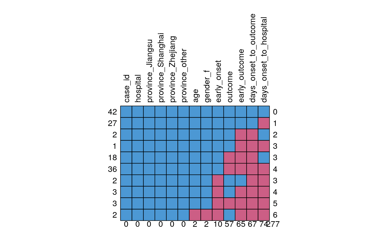
# dataset[, -2] would not work anymore in tibbles
dataset_impute <- mice(data = dataset[, -2],  print = FALSE)
#> Warning: Number of logged events: 150
14.4.1 Generate a dataframe of five imputting strategies
- by default, mice() calculates five (m = 5) imputed data sets
- we can combine them all in one output with the complete(“long”) function
- I did not want to impute missing values in the outcome column, so I have to merge it back in with the imputed data
# c(1,2): case_id, outcome
datasets_complete <- right_join(dataset[, c(1, 2)],
                           complete(dataset_impute, "long"),
                           by = "case_id") %>%
  mutate(.imp = as.factor(.imp)) %>%
  select(-.id) %>%
  glimpse()
#> Rows: 680
#> Columns: 14
#> $ case_id                <dbl> 1, 2, 3, 4, 5, 6, 7, 8, 9, 10, 11, 12, 13, 14,…
#> $ outcome                <fct> Death, Death, Death, NA, Recover, Death, Death…
#> $ .imp                   <fct> 1, 1, 1, 1, 1, 1, 1, 1, 1, 1, 1, 1, 1, 1, 1, 1…
#> $ age                    <dbl> 87, 27, 35, 45, 48, 32, 83, 38, 67, 48, 64, 52…
#> $ hospital               <dbl> 0, 1, 1, 1, 1, 1, 1, 1, 1, 1, 1, 0, 1, 0, 0, 0…
#> $ gender_f               <dbl> 0, 0, 1, 1, 1, 1, 0, 0, 0, 0, 0, 1, 1, 0, 1, 0…
#> $ province_Jiangsu       <dbl> 0, 0, 0, 1, 1, 1, 1, 0, 0, 0, 0, 0, 0, 0, 1, 1…
#> $ province_Shanghai      <dbl> 1, 1, 0, 0, 0, 0, 0, 0, 0, 1, 0, 1, 1, 1, 0, 0…
#> $ province_Zhejiang      <dbl> 0, 0, 0, 0, 0, 0, 0, 1, 1, 0, 1, 0, 0, 0, 0, 0…
#> $ province_other         <dbl> 0, 0, 1, 0, 0, 0, 0, 0, 0, 0, 0, 0, 0, 0, 0, 0…
#> $ days_onset_to_outcome  <dbl> 13, 11, 31, 57, 57, 36, 20, 20, 6, 6, 6, 7, 12…
#> $ days_onset_to_hospital <dbl> 4, 4, 10, 8, 11, 7, 9, 11, 0, 4, 2, 0, 3, 1, 7…
#> $ early_onset            <dbl> 1, 1, 1, 1, 1, 1, 1, 1, 1, 1, 1, 1, 1, 1, 1, 1…
#> $ early_outcome          <dbl> 1, 1, 1, 1, 0, 1, 1, 1, 1, 1, 1, 1, 1, 1, 1, 1…
Let’s compare the distributions of the five different imputed datasets:
14.4.2 plot effect of imputting on features
datasets_complete %>%
  gather(x, y, age:early_outcome) %>%
  ggplot(aes(x = y, fill = .imp, color = .imp)) +
    geom_density(alpha = 0.20) +
  facet_wrap(~ x, ncol = 3, scales = "free") +
    scale_fill_brewer(palette="Set1", na.value = "grey50") +
    scale_color_brewer(palette="Set1", na.value = "grey50") +
    my_theme()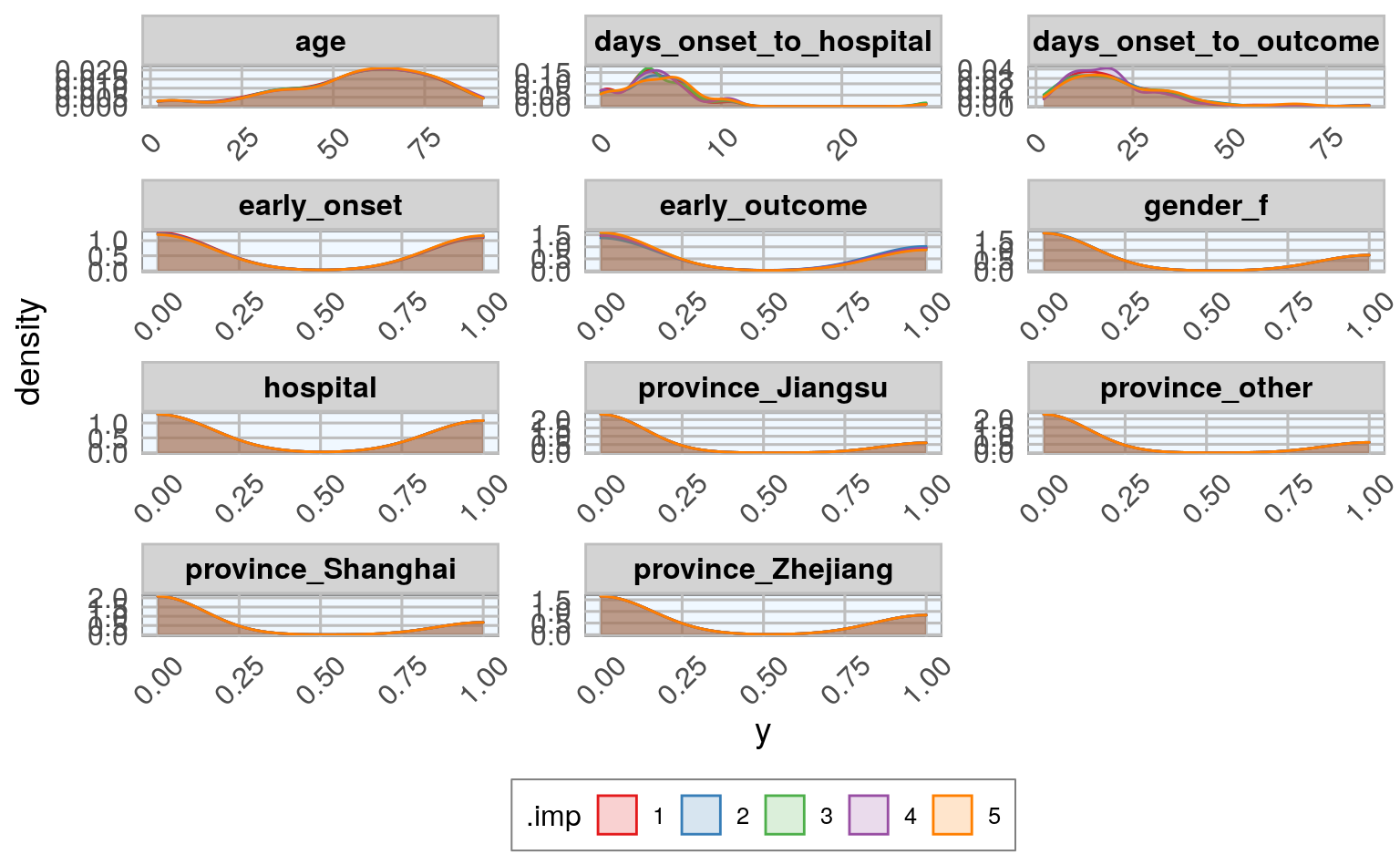
14.5 Test, train and validation data sets
Now, we can go ahead with machine learning!
The dataset contains a few missing values in the outcome column; those will be the test set used for final predictions (see the old blog post for this).
length(which(is.na(datasets_complete$outcome)))
length(which(!is.na(datasets_complete$outcome)))
#> [1] 285
#> [1] 395
train_index <- which(is.na(datasets_complete$outcome))
train_data <- datasets_complete[-train_index, ]
test_data  <- datasets_complete[train_index, -2]       # remove variable outcome
glimpse(train_data)
#> Rows: 395
#> Columns: 14
#> $ case_id                <dbl> 1, 2, 3, 5, 6, 7, 8, 10, 11, 12, 13, 14, 17, 1…
#> $ outcome                <fct> Death, Death, Death, Recover, Death, Death, De…
#> $ .imp                   <fct> 1, 1, 1, 1, 1, 1, 1, 1, 1, 1, 1, 1, 1, 1, 1, 1…
#> $ age                    <dbl> 87, 27, 35, 48, 32, 83, 38, 48, 64, 52, 67, 4,…
#> $ hospital               <dbl> 0, 1, 1, 1, 1, 1, 1, 1, 1, 0, 1, 0, 1, 1, 1, 1…
#> $ gender_f               <dbl> 0, 0, 1, 1, 1, 0, 0, 0, 0, 1, 1, 0, 0, 0, 0, 0…
#> $ province_Jiangsu       <dbl> 0, 0, 0, 1, 1, 1, 0, 0, 0, 0, 0, 0, 0, 0, 0, 0…
#> $ province_Shanghai      <dbl> 1, 1, 0, 0, 0, 0, 0, 1, 0, 1, 1, 1, 1, 1, 1, 0…
#> $ province_Zhejiang      <dbl> 0, 0, 0, 0, 0, 0, 1, 0, 1, 0, 0, 0, 0, 0, 0, 0…
#> $ province_other         <dbl> 0, 0, 1, 0, 0, 0, 0, 0, 0, 0, 0, 0, 0, 0, 0, 1…
#> $ days_onset_to_outcome  <dbl> 13, 11, 31, 57, 36, 20, 20, 6, 6, 7, 12, 10, 1…
#> $ days_onset_to_hospital <dbl> 4, 4, 10, 11, 7, 9, 11, 4, 2, 0, 3, 1, 6, 4, 5…
#> $ early_onset            <dbl> 1, 1, 1, 1, 1, 1, 1, 1, 1, 1, 1, 1, 1, 1, 1, 1…
#> $ early_outcome          <dbl> 1, 1, 1, 0, 1, 1, 1, 1, 1, 1, 1, 1, 1, 1, 0, 1…
# outcome variable removed
glimpse(test_data)
#> Rows: 285
#> Columns: 13
#> $ case_id                <dbl> 4, 9, 15, 16, 22, 28, 31, 32, 38, 39, 40, 41, …
#> $ .imp                   <fct> 1, 1, 1, 1, 1, 1, 1, 1, 1, 1, 1, 1, 1, 1, 1, 1…
#> $ age                    <dbl> 45, 67, 61, 79, 85, 79, 70, 74, 56, 66, 74, 54…
#> $ hospital               <dbl> 1, 1, 0, 0, 1, 0, 0, 0, 0, 1, 1, 1, 1, 0, 1, 0…
#> $ gender_f               <dbl> 1, 0, 1, 0, 0, 0, 0, 0, 0, 0, 0, 1, 0, 0, 0, 1…
#> $ province_Jiangsu       <dbl> 1, 0, 1, 1, 1, 0, 1, 1, 1, 0, 0, 0, 0, 1, 0, 0…
#> $ province_Shanghai      <dbl> 0, 0, 0, 0, 0, 0, 0, 0, 0, 0, 0, 0, 1, 0, 0, 0…
#> $ province_Zhejiang      <dbl> 0, 1, 0, 0, 0, 1, 0, 0, 0, 1, 1, 1, 0, 0, 1, 1…
#> $ province_other         <dbl> 0, 0, 0, 0, 0, 0, 0, 0, 0, 0, 0, 0, 0, 0, 0, 0…
#> $ days_onset_to_outcome  <dbl> 57, 6, 37, 30, 21, 17, 14, 13, 11, 15, 10, 22,…
#> $ days_onset_to_hospital <dbl> 8, 0, 7, 11, 4, 6, 4, 6, 4, 0, 5, 6, 7, 3, 6, …
#> $ early_onset            <dbl> 1, 1, 1, 1, 1, 1, 1, 1, 1, 0, 1, 1, 1, 1, 1, 1…
#> $ early_outcome          <dbl> 1, 1, 1, 1, 1, 1, 1, 1, 1, 1, 1, 1, 1, 0, 1, 1…
The remainder of the data will be used for modeling. Here, I am splitting the data into 70% training and 30% test data.
Because I want to model each imputed dataset separately, I am using the nest() and map() functions.
train_data_nest <- train_data %>%
  group_by(.imp) %>%
  nest() %>%
  print()
#> # A tibble: 5 x 2
#> # Groups:   .imp [5]
#>   .imp  data
#>   <fct> <list>
#> 1 1     <tibble [79 × 13]>
#> 2 2     <tibble [79 × 13]>
#> 3 3     <tibble [79 × 13]>
#> 4 4     <tibble [79 × 13]>
#> 5 5     <tibble [79 × 13]>
# split the training data in validation training and validation test
set.seed(42)
val_data <- train_data_nest %>%
  mutate(val_index = map(data, ~ createDataPartition(.$outcome,
                                                     p = 0.7,
                                               list = FALSE)),
         val_train_data = map2(data, val_index, ~ .x[.y, ]),
         val_test_data  = map2(data, val_index, ~ .x[-.y, ])) %>%
  print()
#> Warning: The `i` argument of ``[`()` can't be a matrix as of tibble 3.0.0.
#> Convert to a vector.
#> This warning is displayed once every 8 hours.
#> Call `lifecycle::last_warnings()` to see where this warning was generated.
#> # A tibble: 5 x 5
#> # Groups:   .imp [5]
#>   .imp  data              val_index          val_train_data    val_test_data
#>   <fct> <list>            <list>             <list>            <list>
#> 1 1     <tibble [79 × 13… <int[,1] [56 × 1]> <tibble [56 × 13… <tibble [23 × 13…
#> 2 2     <tibble [79 × 13… <int[,1] [56 × 1]> <tibble [56 × 13… <tibble [23 × 13…
#> 3 3     <tibble [79 × 13… <int[,1] [56 × 1]> <tibble [56 × 13… <tibble [23 × 13…
#> 4 4     <tibble [79 × 13… <int[,1] [56 × 1]> <tibble [56 × 13… <tibble [23 × 13…
#> 5 5     <tibble [79 × 13… <int[,1] [56 × 1]> <tibble [56 × 13… <tibble [23 × 13…
14.6 Machine Learning algorithms
14.6.1 Random Forest
To make the code tidier, I am first defining the modeling function with the parameters I want.
model_function <- function(df) {
  caret::train(outcome ~ .,
               data = df,
               method = "rf",
               preProcess = c("scale", "center"),
               trControl = trainControl(method = "repeatedcv",
                                        number = 5,
                                        repeats = 3,
                                        verboseIter = FALSE))
}
14.6.2 Add model and prediction to nested dataframe and calculate
Next, I am using the nested tibble from before to map() the model function, predict the outcome and calculate confusion matrices.
14.6.2.1 add model list-column
val_data_model <- val_data %>%
  mutate(model = map(val_train_data, ~ model_function(.x))) %>%
  select(-val_index) %>%
  print()
#> # A tibble: 5 x 5
#> # Groups:   .imp [5]
#>   .imp  data               val_train_data     val_test_data      model
#>   <fct> <list>             <list>             <list>             <list>
#> 1 1     <tibble [79 × 13]> <tibble [56 × 13]> <tibble [23 × 13]> <train>
#> 2 2     <tibble [79 × 13]> <tibble [56 × 13]> <tibble [23 × 13]> <train>
#> 3 3     <tibble [79 × 13]> <tibble [56 × 13]> <tibble [23 × 13]> <train>
#> 4 4     <tibble [79 × 13]> <tibble [56 × 13]> <tibble [23 × 13]> <train>
#> 5 5     <tibble [79 × 13]> <tibble [56 × 13]> <tibble [23 × 13]> <train>
14.6.2.2 add prediction and confusion matrix list-columns
set.seed(42)
val_data_model <- val_data_model %>%
  mutate(
         predict = map2(model, val_test_data, ~
                            data.frame(prediction = predict(.x, .y[, -2]))),
         predict_prob = map2(model, val_test_data, ~
                            data.frame(outcome = .y[, 2],
                            prediction = predict(.x, .y[, -2], type = "prob"))),
         confusion_matrix = map2(val_test_data, predict, ~
                                     confusionMatrix(.x$outcome, .y$prediction)),
         confusion_matrix_tbl = map(confusion_matrix, ~ as.tibble(.x$table))) %>%
  print()
#> # A tibble: 5 x 9
#> # Groups:   .imp [5]
#>   .imp  data  val_train_data val_test_data model predict predict_prob
#>   <fct> <lis> <list>         <list>        <lis> <list>  <list>
#> 1 1     <tib… <tibble [56 ×… <tibble [23 … <tra… <df[,1… <df[,3] [23…
#> 2 2     <tib… <tibble [56 ×… <tibble [23 … <tra… <df[,1… <df[,3] [23…
#> 3 3     <tib… <tibble [56 ×… <tibble [23 … <tra… <df[,1… <df[,3] [23…
#> 4 4     <tib… <tibble [56 ×… <tibble [23 … <tra… <df[,1… <df[,3] [23…
#> 5 5     <tib… <tibble [56 ×… <tibble [23 … <tra… <df[,1… <df[,3] [23…
#> # … with 2 more variables: confusion_matrix <list>, confusion_matrix_tbl <list>
Finally, we have a nested dataframe of 5 rows or cases, one per imputting strategy with its corresponding models and prediction results.
14.7 Comparing accuracy of models
To compare how the different imputations did, I am plotting the confusion matrices:
val_data_model_unnest <- val_data_model %>%
  unnest(confusion_matrix_tbl) %>%
  print()
#> # A tibble: 20 x 11
#> # Groups:   .imp [5]
#>   .imp  data  val_train_data val_test_data model predict predict_prob
#>   <fct> <lis> <list>         <list>        <lis> <list>  <list>
#> 1 1     <tib… <tibble [56 ×… <tibble [23 … <tra… <df[,1… <df[,3] [23…
#> 2 1     <tib… <tibble [56 ×… <tibble [23 … <tra… <df[,1… <df[,3] [23…
#> 3 1     <tib… <tibble [56 ×… <tibble [23 … <tra… <df[,1… <df[,3] [23…
#> 4 1     <tib… <tibble [56 ×… <tibble [23 … <tra… <df[,1… <df[,3] [23…
#> 5 2     <tib… <tibble [56 ×… <tibble [23 … <tra… <df[,1… <df[,3] [23…
#> 6 2     <tib… <tibble [56 ×… <tibble [23 … <tra… <df[,1… <df[,3] [23…
#> # … with 14 more rows, and 4 more variables: confusion_matrix <list>,
#> #   Prediction <chr>, Reference <chr>, n <int>
val_data_model_unnest %>%
  ggplot(aes(x = Prediction, y = Reference, fill = n)) +
    facet_wrap(~ .imp, ncol = 5, scales = "free") +
    geom_tile() +
    my_theme()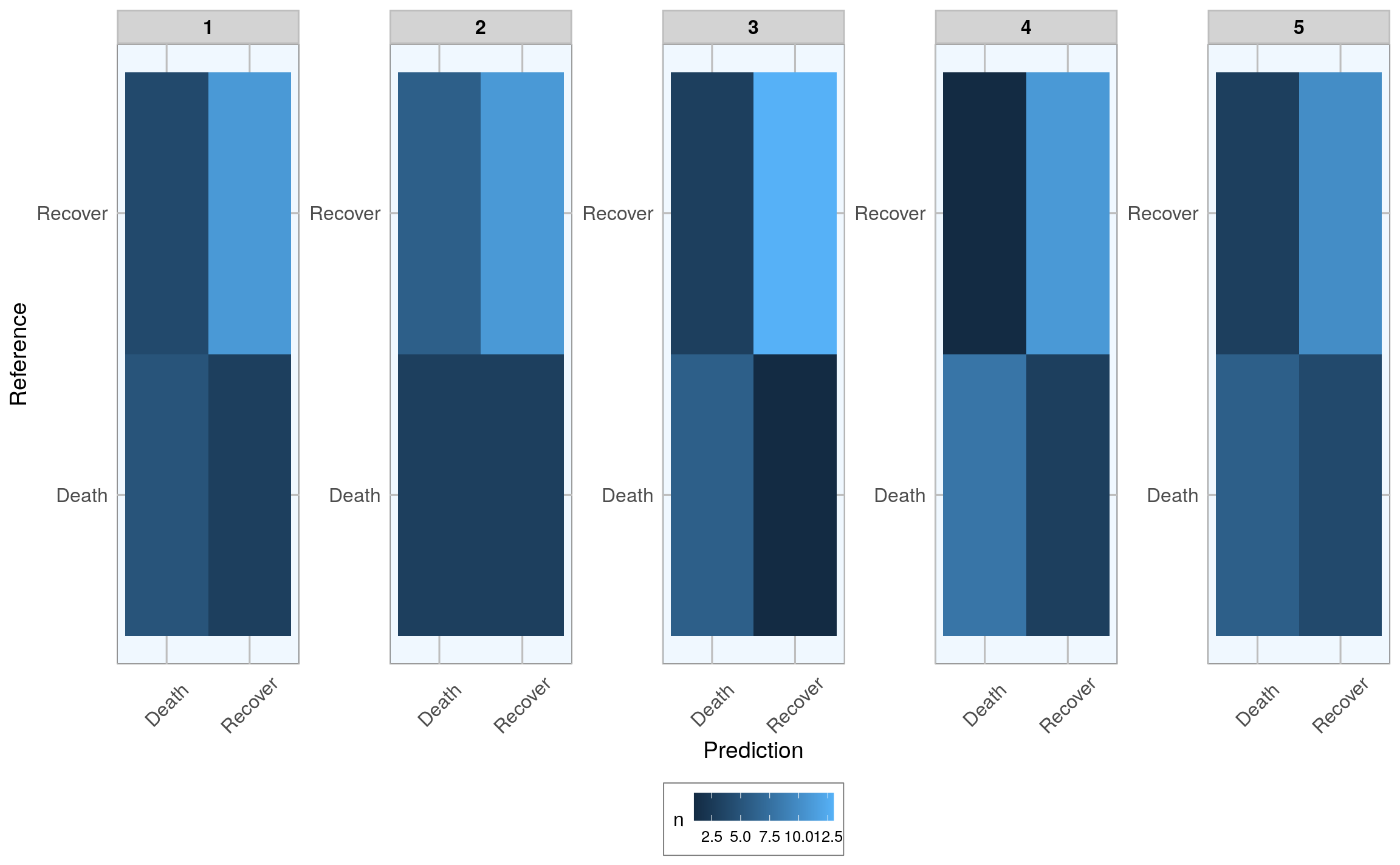
and the prediction probabilities for correct and wrong predictions:
val_data_model_gather <- val_data_model %>%
  unnest(predict_prob) %>%
  gather(x, y, prediction.Death:prediction.Recover) %>%
  print()
#> # A tibble: 230 x 11
#> # Groups:   .imp [5]
#>   .imp  data  val_train_data val_test_data model predict outcome
#>   <fct> <lis> <list>         <list>        <lis> <list>  <fct>
#> 1 1     <tib… <tibble [56 ×… <tibble [23 … <tra… <df[,1… Death
#> 2 1     <tib… <tibble [56 ×… <tibble [23 … <tra… <df[,1… Recover
#> 3 1     <tib… <tibble [56 ×… <tibble [23 … <tra… <df[,1… Death
#> 4 1     <tib… <tibble [56 ×… <tibble [23 … <tra… <df[,1… Death
#> 5 1     <tib… <tibble [56 ×… <tibble [23 … <tra… <df[,1… Recover
#> 6 1     <tib… <tibble [56 ×… <tibble [23 … <tra… <df[,1… Recover
#> # … with 224 more rows, and 4 more variables: confusion_matrix <list>,
#> #   confusion_matrix_tbl <list>, x <chr>, y <dbl>
val_data_model_gather %>%
  ggplot(aes(x = x, y = y, fill = outcome)) +
    facet_wrap(~ .imp, ncol = 5) +
    geom_boxplot() +
    scale_fill_brewer(palette="Set1", na.value = "grey50") +
    my_theme()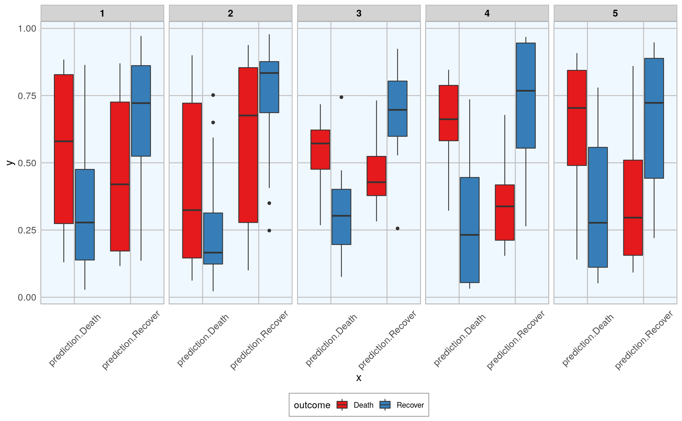
Hope, you found that example interesting and helpful!
sessionInfo()
#> R version 3.6.3 (2020-02-29)
#> Platform: x86_64-pc-linux-gnu (64-bit)
#> Running under: Debian GNU/Linux 10 (buster)
#>
#> Matrix products: default
#> BLAS/LAPACK: /usr/lib/x86_64-linux-gnu/libopenblasp-r0.3.5.so
#>
#> locale:
#>  [1] LC_CTYPE=en_US.UTF-8       LC_NUMERIC=C
#>  [3] LC_TIME=en_US.UTF-8        LC_COLLATE=en_US.UTF-8
#>  [5] LC_MONETARY=en_US.UTF-8    LC_MESSAGES=C
#>  [7] LC_PAPER=en_US.UTF-8       LC_NAME=C
#>  [9] LC_ADDRESS=C               LC_TELEPHONE=C
#> [11] LC_MEASUREMENT=en_US.UTF-8 LC_IDENTIFICATION=C
#>
#> attached base packages:
#> [1] stats     graphics  grDevices utils     datasets  methods   base
#>
#> other attached packages:
#>  [1] caret_6.0-86    lattice_0.20-38 mice_3.8.0      plyr_1.8.6
#>  [5] forcats_0.5.0   stringr_1.4.0   dplyr_0.8.5     purrr_0.3.4
#>  [9] readr_1.3.1     tidyr_1.0.2     tibble_3.0.1    ggplot2_3.3.0
#> [13] tidyverse_1.3.0 outbreaks_1.5.0
#>
#> loaded via a namespace (and not attached):
#>  [1] nlme_3.1-144         fs_1.4.1             lubridate_1.7.8
#>  [4] RColorBrewer_1.1-2   httr_1.4.1           tools_3.6.3
#>  [7] backports_1.1.6      bslib_0.2.2.9000     utf8_1.1.4
#> [10] R6_2.4.1             rpart_4.1-15         DBI_1.1.0
#> [13] colorspace_1.4-1     nnet_7.3-12          withr_2.2.0
#> [16] tidyselect_1.0.0     downlit_0.2.1.9000   compiler_3.6.3
#> [19] cli_2.0.2            rvest_0.3.5          xml2_1.3.2
#> [22] isoband_0.2.1        labeling_0.3         bookdown_0.21.4
#> [25] sass_0.2.0.9005      scales_1.1.0         randomForest_4.6-14
#> [28] rappdirs_0.3.1       digest_0.6.25        rmarkdown_2.5.3
#> [31] pkgconfig_2.0.3      htmltools_0.5.0.9003 dbplyr_1.4.3
#> [34] rlang_0.4.5          readxl_1.3.1         rstudioapi_0.11
#> [37] farver_2.0.3         jquerylib_0.1.2      generics_0.0.2
#> [40] jsonlite_1.6.1       ModelMetrics_1.2.2.2 magrittr_1.5
#> [43] Matrix_1.2-18        Rcpp_1.0.4.6         munsell_0.5.0
#> [46] fansi_0.4.1          lifecycle_0.2.0      stringi_1.4.6
#> [49] pROC_1.16.2          yaml_2.2.1           MASS_7.3-51.5
#> [52] recipes_0.1.10       grid_3.6.3           crayon_1.3.4
#> [55] haven_2.2.0          splines_3.6.3        hms_0.5.3
#> [58] knitr_1.28           pillar_1.4.3         reshape2_1.4.4
#> [61] codetools_0.2-16     stats4_3.6.3         reprex_0.3.0
#> [64] glue_1.4.0           evaluate_0.14        data.table_1.12.8
#> [67] modelr_0.1.6         vctrs_0.2.4          foreach_1.5.0
#> [70] cellranger_1.1.0     gtable_0.3.0         assertthat_0.2.1
#> [73] xfun_0.19.4          gower_0.2.1          prodlim_2019.11.13
#> [76] broom_0.5.6          e1071_1.7-3          class_7.3-15
#> [79] survival_3.1-8       timeDate_3043.102    iterators_1.0.12
#> [82] lava_1.6.7           ellipsis_0.3.0       ipred_0.9-9