37 Comparing Multiple Regression vs a Neural Network
- Dataset:
diamonds - Algorithms:
- Neural Networks (
RSNNS) - Multiple Regression
- Neural Networks (
37.1 Introduction
Source: http://beyondvalence.blogspot.com/2014/04/r-comparing-multiple-and-neural-network.html
Here we will compare and evaluate the results from multiple regression and a neural network on the diamonds data set from the ggplot2 package in R. Consisting of 53,940 observations with 10 variables, diamonds contains data on the carat, cut, color, clarity, price, and diamond dimensions. These variables have a particular effect on price, and we would like to see if they can predict the price of various diamonds.
library(ggplot2)
library(RSNNS)
#> Loading required package: Rcpp
library(MASS)
library(caret)
#> Loading required package: lattice
#>
#> Attaching package: 'caret'
#> The following objects are masked from 'package:RSNNS':
#>
#>     confusionMatrix, train
# library(diamonds)

head(diamonds)
#> # A tibble: 6 x 10
#>   carat cut       color clarity depth table price     x     y     z
#>   <dbl> <ord>     <ord> <ord>   <dbl> <dbl> <int> <dbl> <dbl> <dbl>
#> 1 0.23  Ideal     E     SI2      61.5    55   326  3.95  3.98  2.43
#> 2 0.21  Premium   E     SI1      59.8    61   326  3.89  3.84  2.31
#> 3 0.23  Good      E     VS1      56.9    65   327  4.05  4.07  2.31
#> 4 0.290 Premium   I     VS2      62.4    58   334  4.2   4.23  2.63
#> 5 0.31  Good      J     SI2      63.3    58   335  4.34  4.35  2.75
#> 6 0.24  Very Good J     VVS2     62.8    57   336  3.94  3.96  2.48
dplyr::glimpse(diamonds)
#> Rows: 53,940
#> Columns: 10
#> $ carat   <dbl> 0.23, 0.21, 0.23, 0.29, 0.31, 0.24, 0.24, 0.26, 0.22, 0.23, 0…
#> $ cut     <ord> Ideal, Premium, Good, Premium, Good, Very Good, Very Good, Ve…
#> $ color   <ord> E, E, E, I, J, J, I, H, E, H, J, J, F, J, E, E, I, J, J, J, I…
#> $ clarity <ord> SI2, SI1, VS1, VS2, SI2, VVS2, VVS1, SI1, VS2, VS1, SI1, VS1,…
#> $ depth   <dbl> 61.5, 59.8, 56.9, 62.4, 63.3, 62.8, 62.3, 61.9, 65.1, 59.4, 6…
#> $ table   <dbl> 55, 61, 65, 58, 58, 57, 57, 55, 61, 61, 55, 56, 61, 54, 62, 5…
#> $ price   <int> 326, 326, 327, 334, 335, 336, 336, 337, 337, 338, 339, 340, 3…
#> $ x       <dbl> 3.95, 3.89, 4.05, 4.20, 4.34, 3.94, 3.95, 4.07, 3.87, 4.00, 4…
#> $ y       <dbl> 3.98, 3.84, 4.07, 4.23, 4.35, 3.96, 3.98, 4.11, 3.78, 4.05, 4…
#> $ z       <dbl> 2.43, 2.31, 2.31, 2.63, 2.75, 2.48, 2.47, 2.53, 2.49, 2.39, 2…
The cut, color, and clarity variables are factors, and must be treated as dummy variables in multiple and neural network regressions. Let us start with multiple regression.
37.2 Multiple Regression
First we ready a Multiple Regression by sampling the rows to randomize the observations, and then create a sample index of 0’s and 1’s to separate the training and test sets. Note that the depth and table columns (5, 6) are removed because they are linear combinations of the dimensions, x, y, and z. See that the observations in the training and test sets approximate 70% and 30% of the total observations, from which we sampled and set the probabilities.
set.seed(1234567)
diamonds <- diamonds[sample(1:nrow(diamonds), nrow(diamonds)),]
d.index = sample(0:1, nrow(diamonds), prob=c(0.3, 0.7), rep = TRUE)
d.train <- diamonds[d.index==1, c(-5,-6)]
d.test <- diamonds[d.index==0, c(-5,-6)]
dim(d.train)
#> [1] 37502     8
dim(d.test)
#> [1] 16438     8
Now we move into the next stage with multiple regression via the train() function from the caret library, instead of the regular lm() function. We specify the predictors, the response variable (price), the “lm” method, and the cross validation resampling method.
x <- d.train[,-5]
y <- as.numeric(d.train[,5]$price)

ds.lm <- caret::train(x, y, method = "lm",
                      trainControl = trainControl(method = "cv"))
#> Warning: Setting row names on a tibble is deprecated.
#> Warning: In lm.fit(x, y, offset = offset, singular.ok = singular.ok, ...) :
#>  extra argument 'trainControl' will be disregarded
#> Warning: Setting row names on a tibble is deprecated.
#> Warning: In lm.fit(x, y, offset = offset, singular.ok = singular.ok, ...) :
#>  extra argument 'trainControl' will be disregarded
#> Warning: Setting row names on a tibble is deprecated.
#> Warning: In lm.fit(x, y, offset = offset, singular.ok = singular.ok, ...) :
#>  extra argument 'trainControl' will be disregarded
#> Warning: Setting row names on a tibble is deprecated.
#> Warning: In lm.fit(x, y, offset = offset, singular.ok = singular.ok, ...) :
#>  extra argument 'trainControl' will be disregarded
#> Warning: Setting row names on a tibble is deprecated.
#> Warning: In lm.fit(x, y, offset = offset, singular.ok = singular.ok, ...) :
#>  extra argument 'trainControl' will be disregarded
#> Warning: Setting row names on a tibble is deprecated.
#> Warning: In lm.fit(x, y, offset = offset, singular.ok = singular.ok, ...) :
#>  extra argument 'trainControl' will be disregarded
#> Warning: Setting row names on a tibble is deprecated.
#> Warning: In lm.fit(x, y, offset = offset, singular.ok = singular.ok, ...) :
#>  extra argument 'trainControl' will be disregarded
#> Warning: Setting row names on a tibble is deprecated.
#> Warning: In lm.fit(x, y, offset = offset, singular.ok = singular.ok, ...) :
#>  extra argument 'trainControl' will be disregarded
#> Warning: Setting row names on a tibble is deprecated.
#> Warning: In lm.fit(x, y, offset = offset, singular.ok = singular.ok, ...) :
#>  extra argument 'trainControl' will be disregarded
#> Warning: Setting row names on a tibble is deprecated.
#> Warning: In lm.fit(x, y, offset = offset, singular.ok = singular.ok, ...) :
#>  extra argument 'trainControl' will be disregarded
#> Warning: Setting row names on a tibble is deprecated.
#> Warning: In lm.fit(x, y, offset = offset, singular.ok = singular.ok, ...) :
#>  extra argument 'trainControl' will be disregarded
#> Warning: Setting row names on a tibble is deprecated.
#> Warning: In lm.fit(x, y, offset = offset, singular.ok = singular.ok, ...) :
#>  extra argument 'trainControl' will be disregarded
#> Warning: Setting row names on a tibble is deprecated.
#> Warning: In lm.fit(x, y, offset = offset, singular.ok = singular.ok, ...) :
#>  extra argument 'trainControl' will be disregarded
#> Warning: Setting row names on a tibble is deprecated.
#> Warning: In lm.fit(x, y, offset = offset, singular.ok = singular.ok, ...) :
#>  extra argument 'trainControl' will be disregarded
#> Warning: Setting row names on a tibble is deprecated.
#> Warning: In lm.fit(x, y, offset = offset, singular.ok = singular.ok, ...) :
#>  extra argument 'trainControl' will be disregarded
#> Warning: Setting row names on a tibble is deprecated.
#> Warning: In lm.fit(x, y, offset = offset, singular.ok = singular.ok, ...) :
#>  extra argument 'trainControl' will be disregarded
#> Warning: Setting row names on a tibble is deprecated.
#> Warning: In lm.fit(x, y, offset = offset, singular.ok = singular.ok, ...) :
#>  extra argument 'trainControl' will be disregarded
#> Warning: Setting row names on a tibble is deprecated.
#> Warning: In lm.fit(x, y, offset = offset, singular.ok = singular.ok, ...) :
#>  extra argument 'trainControl' will be disregarded
#> Warning: Setting row names on a tibble is deprecated.
#> Warning: In lm.fit(x, y, offset = offset, singular.ok = singular.ok, ...) :
#>  extra argument 'trainControl' will be disregarded
#> Warning: Setting row names on a tibble is deprecated.
#> Warning: In lm.fit(x, y, offset = offset, singular.ok = singular.ok, ...) :
#>  extra argument 'trainControl' will be disregarded
#> Warning: Setting row names on a tibble is deprecated.
#> Warning: In lm.fit(x, y, offset = offset, singular.ok = singular.ok, ...) :
#>  extra argument 'trainControl' will be disregarded
#> Warning: Setting row names on a tibble is deprecated.
#> Warning: In lm.fit(x, y, offset = offset, singular.ok = singular.ok, ...) :
#>  extra argument 'trainControl' will be disregarded
#> Warning: Setting row names on a tibble is deprecated.
#> Warning: In lm.fit(x, y, offset = offset, singular.ok = singular.ok, ...) :
#>  extra argument 'trainControl' will be disregarded
#> Warning: Setting row names on a tibble is deprecated.
#> Warning: In lm.fit(x, y, offset = offset, singular.ok = singular.ok, ...) :
#>  extra argument 'trainControl' will be disregarded
#> Warning: Setting row names on a tibble is deprecated.
#> Warning: In lm.fit(x, y, offset = offset, singular.ok = singular.ok, ...) :
#>  extra argument 'trainControl' will be disregarded
#> Warning: Setting row names on a tibble is deprecated.
#> Warning: In lm.fit(x, y, offset = offset, singular.ok = singular.ok, ...) :
#>  extra argument 'trainControl' will be disregarded
ds.lm
#> Linear Regression
#>
#> 37502 samples
#>     7 predictor
#>
#> No pre-processing
#> Resampling: Bootstrapped (25 reps)
#> Summary of sample sizes: 37502, 37502, 37502, 37502, 37502, 37502, ...
#> Resampling results:
#>
#>   RMSE  Rsquared  MAE
#>   1140  0.919     745
#>
#> Tuning parameter 'intercept' was held constant at a value of TRUE
When we call the train(ed) object, we can see the attributes of the training set, resampling, sample sizes, and the results. Note the root mean square error value of 1150. Will that be low enough to take down heavy weight TEAM: Neural Network? Below we visualize the training diamond prices and the predicted prices with ggplot().
library(dplyr)
#>
#> Attaching package: 'dplyr'
#> The following object is masked from 'package:MASS':
#>
#>     select
#> The following objects are masked from 'package:stats':
#>
#>     filter, lag
#> The following objects are masked from 'package:base':
#>
#>     intersect, setdiff, setequal, union

data.frame(obs = y, pred = ds.lm$finalModel$fitted.values) %>%
  ggplot(aes(x = obs, y = pred)) +
  geom_point(alpha=0.1) +
  geom_abline(color="blue") +
  labs(title="Diamond train price", x="observed", y="predicted")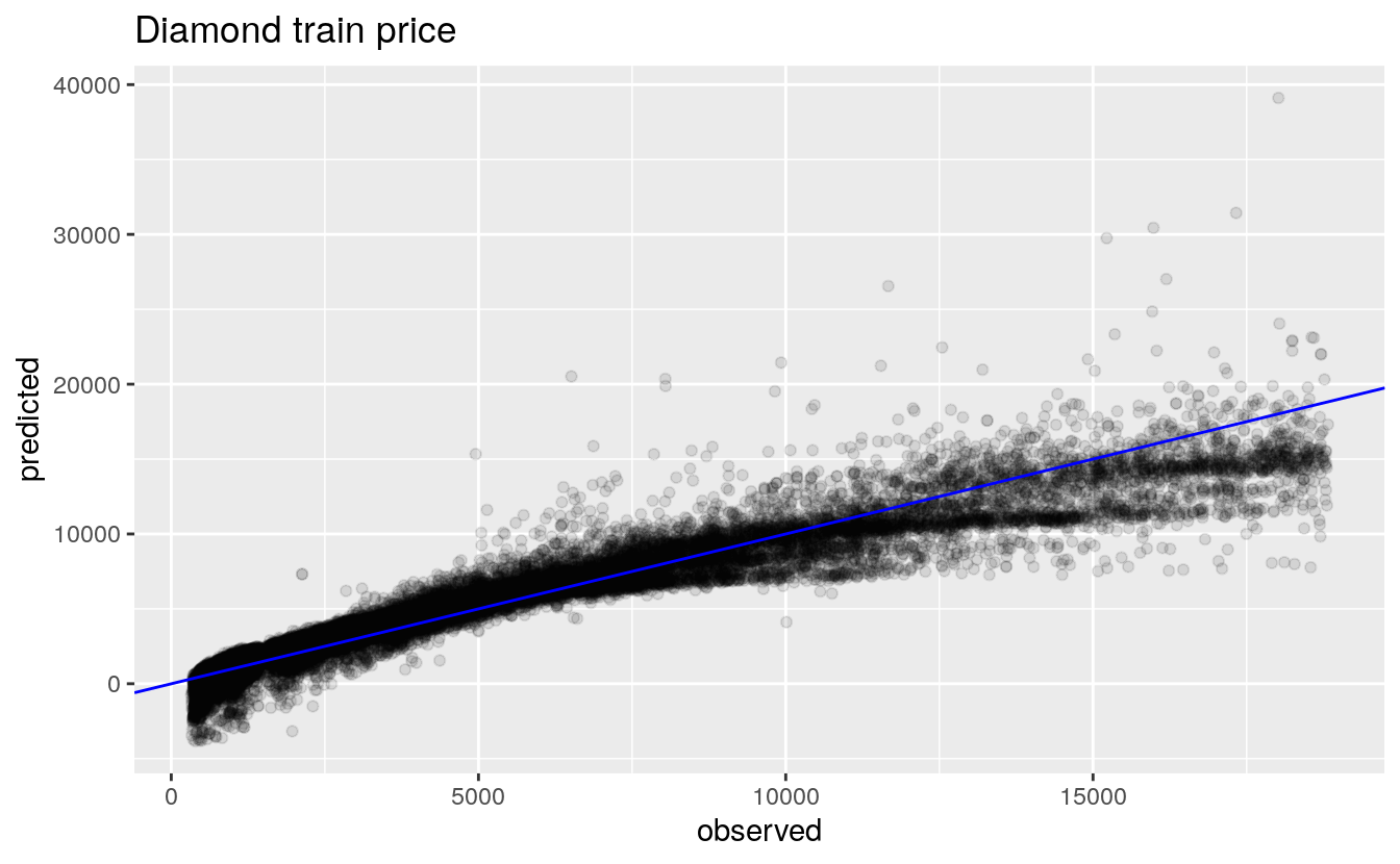
We see from the axis, the predicted prices have some high values compared to the actual prices. Also, there are predicted prices below 0, which cannot be possible in the observed, which will set TEAM: Multiple Regression back a few points.
Next we use ggplot() again to visualize the predicted and observed diamond prices from the test data, which did not train the linear regression model.
# predict on test set
ds.lm.p <- predict(ds.lm, d.test[,-5], type="raw")

# compare observed vs predicted prices in the test set
data.frame(obs = d.test[,5]$price, pred = ds.lm.p) %>%
  ggplot(aes(x = obs, y = pred)) +
  geom_point(alpha=0.1) +
  geom_abline(color="blue")+
  labs("Diamond Test Price", x="observed", y="predicted")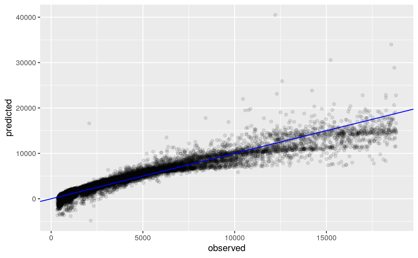
Similar to the training prices plot, we see here in the test prices that the model over predicts larger values and also predicted negative price values. In order for the Multiple Regression to win, the Neural Network has to have more wild prediction values.
Lastly, we calculate the root mean square error, by taking the mean of the squared difference between the predicted and observed diamond prices. The resulting RMSE is 1110.843, similar to the RMSE of the training set.
ds.lm.mse <- (1 / nrow(d.test)) * sum((ds.lm.p - d.test[,5])^2)
lm.rmse <- sqrt(ds.lm.mse)
lm.rmse
#> [1] 1168
Below is a detailed output of the model summary, with the coefficients and residuals. Observe how carat is the best predictor, with the highest t value at 191.7, with every increase in 1 carat holding all other variables equal, results in a 10,873 dollar increase in value. As we look at the factor variables, we do not see a reliable increase in coefficients with increases in level value.
summary(ds.lm)
#>
#> Call:
#> lm(formula = .outcome ~ ., data = dat, trainControl = ..1)
#>
#> Residuals:
#>    Min     1Q Median     3Q    Max
#> -21090   -598   -183    378  10778
#>
#> Coefficients:
#>             Estimate Std. Error t value Pr(>|t|)
#> (Intercept)     3.68      94.63    0.04   0.9690
#> carat       11142.68      57.43  194.02  < 2e-16 ***
#> cut.L         767.70      24.31   31.58  < 2e-16 ***
#> cut.Q        -336.63      21.41  -15.72  < 2e-16 ***
#> cut.C         157.31      18.81    8.36  < 2e-16 ***
#> cut^4         -22.81      14.78   -1.54   0.1228
#> color.L     -1950.28      20.66  -94.42  < 2e-16 ***
#> color.Q      -665.60      18.82  -35.37  < 2e-16 ***
#> color.C      -147.16      17.61   -8.36  < 2e-16 ***
#> color^4        44.64      16.20    2.76   0.0059 **
#> color^5       -91.21      15.32   -5.95  2.7e-09 ***
#> color^6       -54.74      13.92   -3.93  8.5e-05 ***
#> clarity.L    4115.45      36.68  112.19  < 2e-16 ***
#> clarity.Q   -1959.71      34.33  -57.09  < 2e-16 ***
#> clarity.C     990.60      29.29   33.83  < 2e-16 ***
#> clarity^4    -370.82      23.30  -15.92  < 2e-16 ***
#> clarity^5     240.60      18.91   12.72  < 2e-16 ***
#> clarity^6      -7.99      16.37   -0.49   0.6253
#> clarity^7      80.62      14.48    5.57  2.6e-08 ***
#> x           -1400.26      95.70  -14.63  < 2e-16 ***
#> y             545.42      94.57    5.77  8.1e-09 ***
#> z            -190.86      31.20   -6.12  9.6e-10 ***
#> ---
#> Signif. codes:  0 '***' 0.001 '**' 0.01 '*' 0.05 '.' 0.1 ' ' 1
#>
#> Residual standard error: 1130 on 37480 degrees of freedom
#> Multiple R-squared:  0.92,   Adjusted R-squared:  0.92
#> F-statistic: 2.05e+04 on 21 and 37480 DF,  p-value: <2e-16
Now we move on to the neural network regression.
37.3 Neural Network
Because neural networks operate in terms of 0 to 1, or -1 to 1, we must first normalize the price variable to 0 to 1, making the lowest value 0 and the highest value 1. We accomplished this using the normalizeData() function. Save the price output in order to revert the normalization after training the data. Also, we take the factor variables and turn them into numeric labels using toNumericClassLabels(). Below we see the normalized prices before they are split into a training and test set with splitForTrainingAndTest() function.
diamonds[,3] <- toNumericClassLabels(diamonds[,3]$color)
diamonds[,4] <- toNumericClassLabels(diamonds[,4]$clarity)
prices <- normalizeData(diamonds[,7], type="0_1")
head(prices)
#>        [,1]
#> [1,] 0.0841
#> [2,] 0.1491
#> [3,] 0.0237
#> [4,] 0.3247
#> [5,] 0.0280
#> [6,] 0.0252
dsplit <- splitForTrainingAndTest(diamonds[, c(-2,-5,-6,-7,-9,-10)], prices, ratio=0.3)Now the Neural Network are ready for the multi-layer perceptron (MLP) regression. We define the training inputs (predictor variables) and targets (prices), the size of the layer (5), the incremented learning parameter (0.1), the max iterations (100 epochs), and also the test input/targets.
# mlp model
d.nn <- mlp(dsplit$inputsTrain,
            dsplit$targetsTrain,
            size = c(5), learnFuncParams = c(0.1), maxit=100,
            inputsTest = dsplit$inputsTest,
            targetsTest = dsplit$targetsTest,
            metric = "RMSE",
            linout = FALSE)
If you spectators have dealt with mlp() before, you know the summary output can be quite lenghty, so it is omitted (we dislike commercials too). We move to the visual description of the MLP model with the iterative sum of square error for the training and test sets. Additionally, we plot the regression error (predicted vs observed) for the training and test prices.
Time for the Neural Network so show off its statistical muscles! First up, we have the iterative sum of square error for each epoch, noting that we specified a maximum of 100 in the MLP model. We see an immediate drop in the SSE with the first few iterations, with the SSE leveling out around 50. The test SSE, in red, fluctuations just above 50 as well. Since the SSE began to plateau, the model fit well but not too well, since we want to avoid over fitting the model. So 100 iterations was a good choice.
# SSE error
plotIterativeError(d.nn, main = "Diamonds RSNNS-SSE")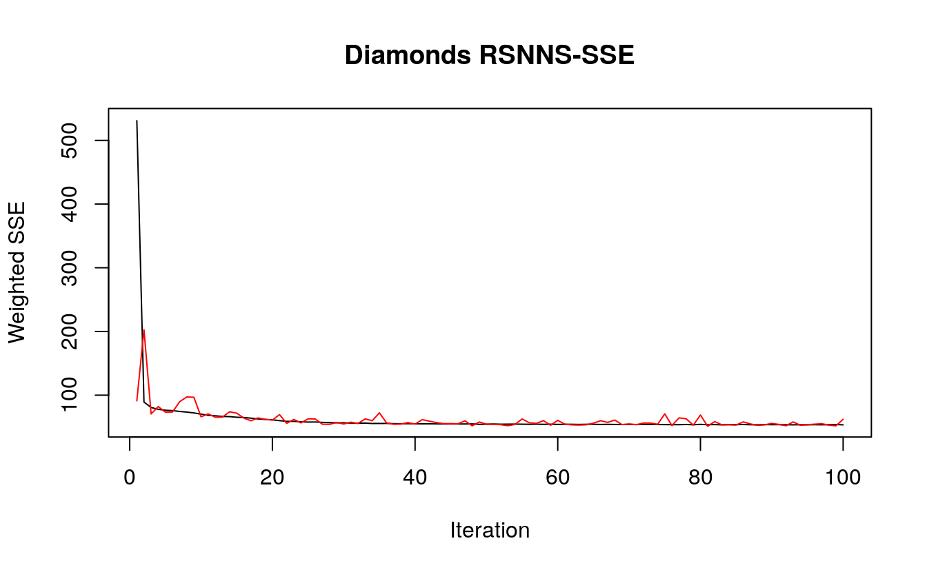
Second, we observe the regression plot with the fitted (predicted) and target (observed) prices from the training set. The prices fit reasonably well, and we see the red model regression line close to the black (y=x) optimal line. Note that some middle prices were over predicted by the model, and there were no negative prices, unlike the linear regression model.
# regression  errors
plotRegressionError(dsplit$targetsTrain, d.nn$fitted.values,
                    main = "Diamonds Training Fit")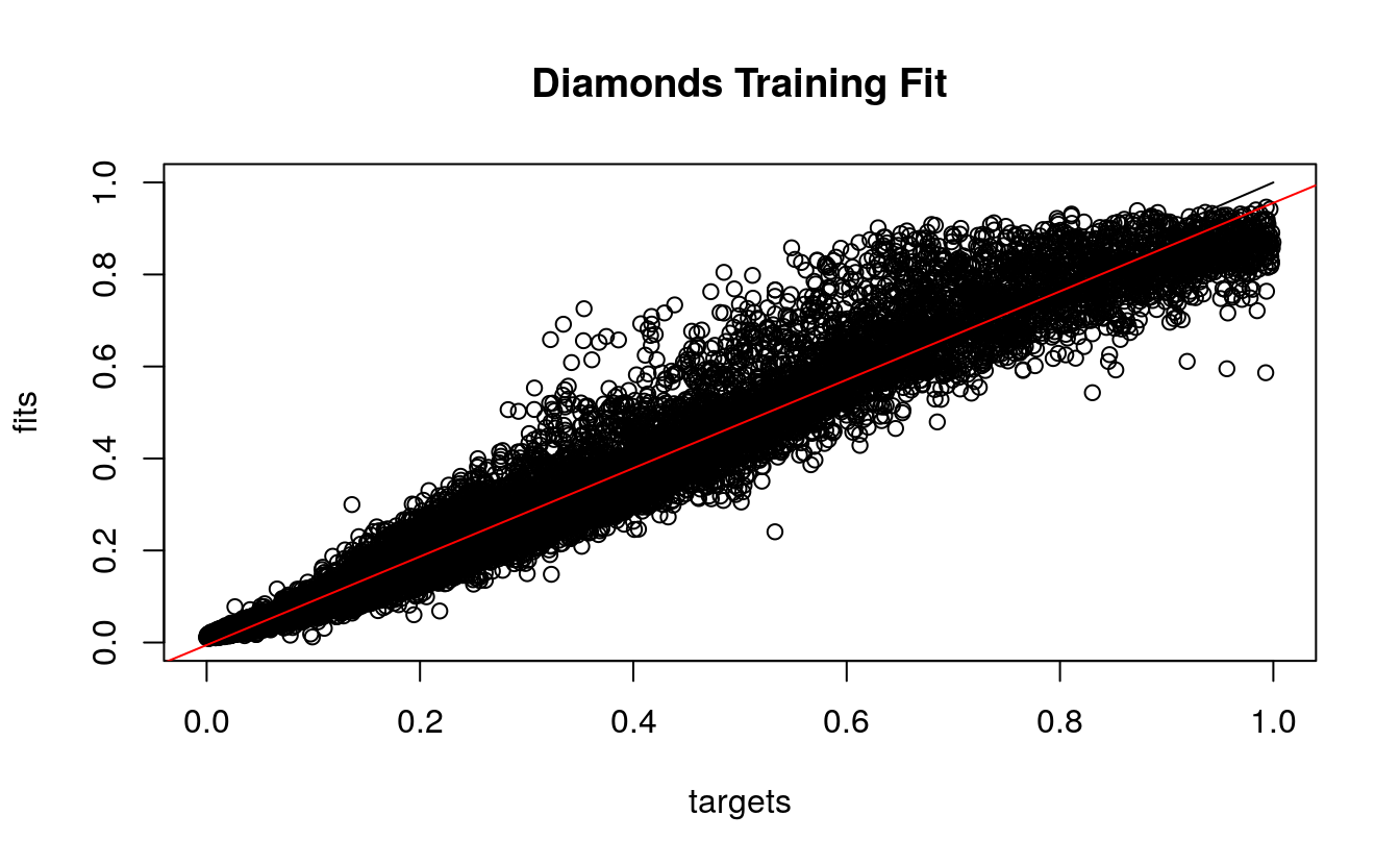
Third, we look at the predicted and observed prices from the test set. Again the red regression line approximates the optimal black line, and more price values were over predicted by the model. Again, there are no negative predicted prices, a good sign.
plotRegressionError(dsplit$targetsTest, d.nn$fittedTestValues,
                    main = "Diamonds Test Fit")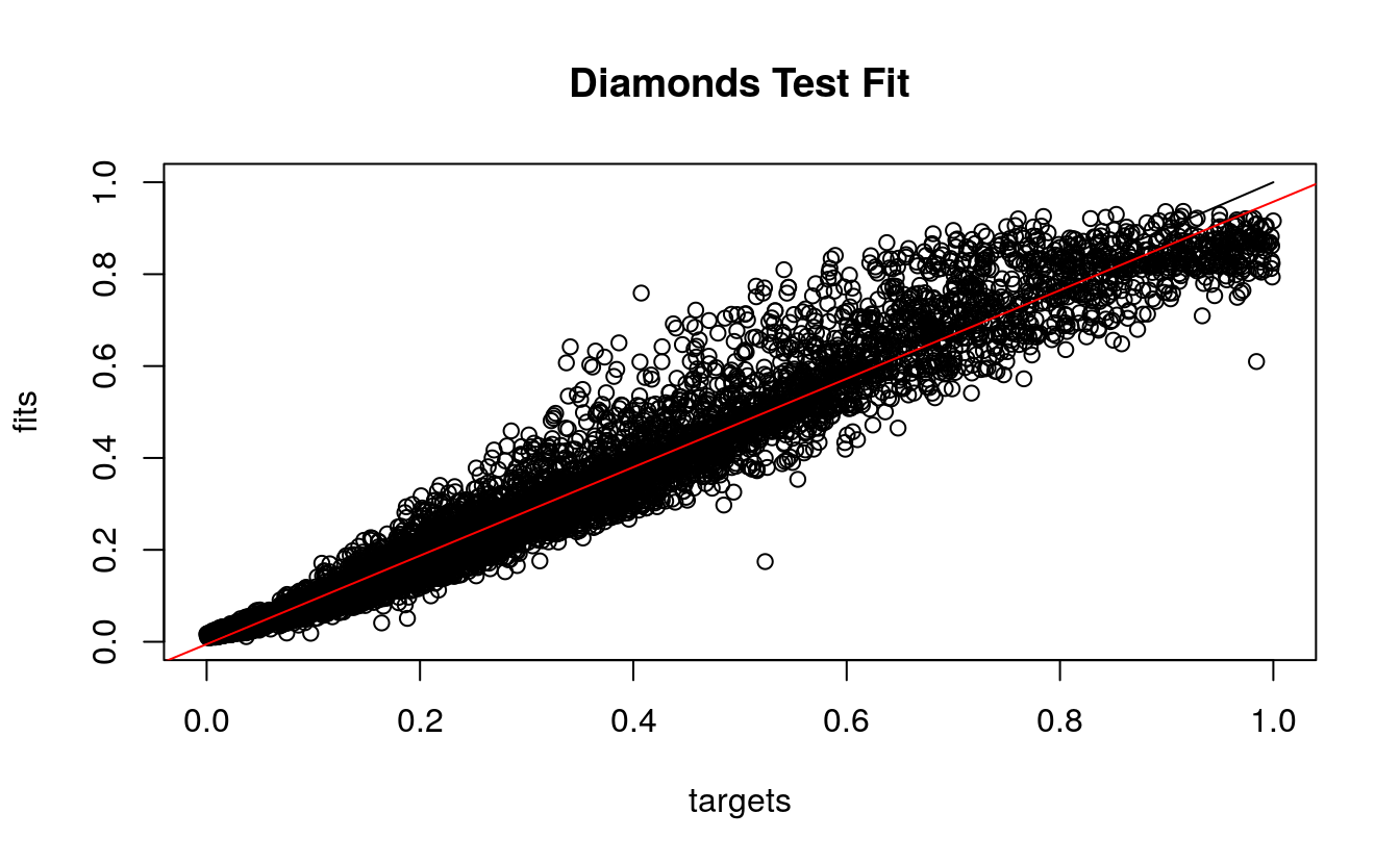
Now we calculate the RMSE for the training set, which we get 692.5155. This looks promising for the Neural Network!
# train set
train.pred <- denormalizeData(d.nn$fitted.values,
                              getNormParameters(prices))

train.obs <- denormalizeData(dsplit$targetsTrain,
                             getNormParameters(prices))

train.mse <- (1 / nrow(dsplit$inputsTrain)) * sum((train.pred - train.obs)^2)

rsnns.train.rmse <- sqrt(train.mse)
rsnns.train.rmse
#> [1] 739
Naturally we want to calculate the RMSE for the test set, but note that in the real world, we would not have the luxury of knowing the real test values. We arrive at 679.5265.
# test set
test.pred <- denormalizeData(d.nn$fittedTestValues,
                             getNormParameters(prices))

test.obs <- denormalizeData(dsplit$targetsTest,
                            getNormParameters(prices))

test.mse <- (1 / nrow(dsplit$inputsTest)) * sum((test.pred - test.obs)^2)

rsnns.test.rmse <- sqrt(test.mse)
rsnns.test.rmse
#> [1] 751
Which model was better in predicting the diamond price? The linear regression model with 10 fold cross validation, or the multi-layer perceptron model with 5 nodes run to 100 iterations? Who won the rumble?
RUMBLE RESULTS
From calculating the two RMSE’s from the training and test sets for the two TEAMS, we wrap them in a list. We named the TEAM: Multiple Regression as linear, and the TEAM: Neural Network regression as neural.
# aggregate all rmse
d.rmse <- list(linear.train = ds.lm$results$RMSE,
               linear.test = lm.rmse,
               neural.train = rsnns.train.rmse,
               neural.test = rsnns.test.rmse)
Below we can evaluate the models from their RMSE values.
d.rmse
#> $linear.train
#> [1] 1140
#>
#> $linear.test
#> [1] 1168
#>
#> $neural.train
#> [1] 739
#>
#> $neural.test
#> [1] 751
Looking at the training RMSE first, we see a clear difference as the linear RMSE was 66% larger than the neural RMSE, at 1,152.393 versus 692.5155. Peeking into the test sets, we have a similar 63% larger linear RMSE than the neural RMSE, with 1,110.843 and 679.5265 respectively. TEAM: Neural Network begins to gain the upper hand in the evaluation round.
One important difference between the two models was the range of the predictions. Recall from both training and test plots that the linear regression model predicted negative price values, whereas the MLP model predicted only positive prices. This is a devastating blow to the Multiple Regression. Also, the over-prediction of prices existed in both models, however the linear regression model over predicted those middle values higher the anticipated maximum price values.
Sometimes the simple models are optimal, and other times more complicated models are better. This time, the neural network model prevailed in predicting diamond prices.