39 Credit Scoring with neuralnet
39.1 Introduction
Source: https://www.r-bloggers.com/using-neural-networks-for-credit-scoring-a-simple-example/
39.2 Motivation
Credit scoring is the practice of analysing a persons background and credit application in order to assess the creditworthiness of the person. One can take numerous approaches on analysing this creditworthiness. In the end it basically comes down to first selecting the correct independent variables (e.g. income, age, gender) that lead to a given level of creditworthiness.
In other words: creditworthiness = f(income, age, gender, …).
A creditscoring system can be represented by linear regression, logistic regression, machine learning or a combination of these. Neural networks are situated in the domain of machine learning. The following is an strongly simplified example. The actual procedure of building a credit scoring system is much more complex and the resulting model will most likely not consist of solely or even a neural network.
If you’re unsure on what a neural network exactly is, I find this a good place to start.
For this example the R package neuralnet is used, for a more in-depth view on the exact workings of the package see neuralnet: Training of Neural Networks by F. Günther and S. Fritsch.
39.3 load the data
Dataset downloaded: https://gist.github.com/Bart6114/8675941#file-creditset-csv
set.seed(1234567890)

library(neuralnet)

dataset <- read.csv(file.path(data_raw_dir, "creditset.csv"))
head(dataset)
#>   clientid income  age   loan      LTI default10yr
#> 1        1  66156 59.0 8106.5 0.122537           0
#> 2        2  34415 48.1 6564.7 0.190752           0
#> 3        3  57317 63.1 8021.0 0.139940           0
#> 4        4  42710 45.8 6103.6 0.142911           0
#> 5        5  66953 18.6 8770.1 0.130989           1
#> 6        6  24904 57.5   15.5 0.000622           0
names(dataset)
#> [1] "clientid"    "income"      "age"         "loan"        "LTI"
#> [6] "default10yr"
summary(dataset)
#>     clientid        income           age            loan            LTI
#>  Min.   :   1   Min.   :20014   Min.   :18.1   Min.   :    1   Min.   :0.0000
#>  1st Qu.: 501   1st Qu.:32796   1st Qu.:29.1   1st Qu.: 1940   1st Qu.:0.0479
#>  Median :1000   Median :45789   Median :41.4   Median : 3975   Median :0.0994
#>  Mean   :1000   Mean   :45332   Mean   :40.9   Mean   : 4444   Mean   :0.0984
#>  3rd Qu.:1500   3rd Qu.:57791   3rd Qu.:52.6   3rd Qu.: 6432   3rd Qu.:0.1476
#>  Max.   :2000   Max.   :69996   Max.   :64.0   Max.   :13766   Max.   :0.1999
#>   default10yr
#>  Min.   :0.000
#>  1st Qu.:0.000
#>  Median :0.000
#>  Mean   :0.142
#>  3rd Qu.:0.000
#>  Max.   :1.000
# distribution of defaults
table(dataset$default10yr)
#>
#>    0    1
#> 1717  283
min(dataset$LTI)
#> [1] 4.91e-05
plot(jitter(dataset$default10yr, 1) ~ jitter(dataset$LTI, 2))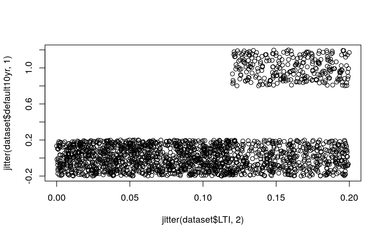
# convert LTI continuous variable to categorical
dataset$LTIrng <- cut(dataset$LTI, breaks = 10)
unique(dataset$LTIrng)
#>  [1] (0.12,0.14]      (0.18,0.2]       (0.14,0.16]      (-0.000151,0.02]
#>  [5] (0.1,0.12]       (0.04,0.06]      (0.06,0.08]      (0.08,0.1]
#>  [9] (0.16,0.18]      (0.02,0.04]
#> 10 Levels: (-0.000151,0.02] (0.02,0.04] (0.04,0.06] (0.06,0.08] ... (0.18,0.2]
plot(dataset$LTIrng, dataset$default10yr)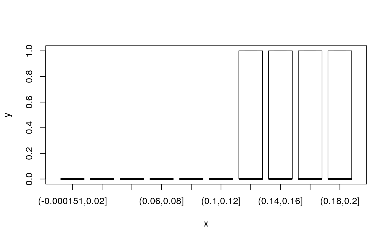
# what age and LTI is more likely to default
library(ggplot2)

ggplot(dataset, aes(x = age, y = LTI, col = default10yr)) +
    geom_point()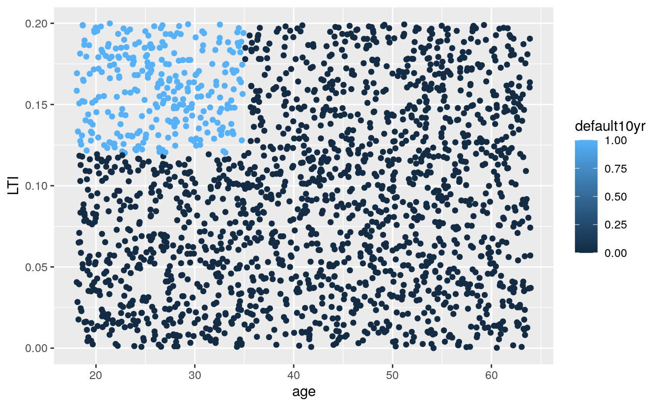
# what age and loan size is more likely to default
library(ggplot2)

ggplot(dataset, aes(x = age, y = loan, col = default10yr)) +
    geom_point()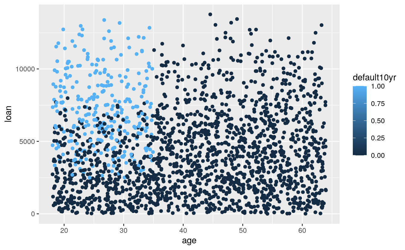
39.4 Objective
The dataset contains information on different clients who received a loan at least 10 years ago. The variables income (yearly), age, loan (size in euros) and LTI (the loan to yearly income ratio) are available. Our goal is to devise a model which predicts, based on the input variables LTI and age, whether or not a default will occur within 10 years.
39.5 Steps
The dataset will be split up in a subset used for training the neural network and another set used for testing. As the ordering of the dataset is completely random, we do not have to extract random rows and can just take the first x rows.
## extract a set to train the NN
trainset <- dataset[1:800, ]

## select the test set
testset <- dataset[801:2000, ]
39.5.1 Build the neural network
Now we’ll build a neural network with 4 hidden nodes (a neural network is comprised of an input, hidden and output nodes). The number of nodes is chosen here without a clear method, however there are some rules of thumb. The lifesign option refers to the verbosity. The ouput is not linear and we will use a threshold value of 10%. The neuralnet package uses resilient backpropagation with weight backtracking as its standard algorithm.
## build the neural network (NN)
creditnet <- neuralnet(default10yr ~ LTI + age, trainset,
                       hidden = 4,
                       lifesign = "minimal",
                       linear.output = FALSE,
                       threshold = 0.1)
#> hidden: 4    thresh: 0.1    rep: 1/1    steps:   44487   error: 0.20554  time: 8 secs
The neuralnet package also has the possibility to visualize the generated model and show the found weights.
## plot the NN
plot(creditnet, rep = "best")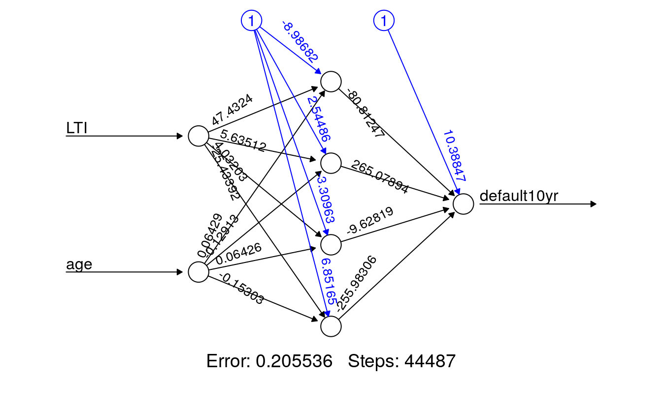
39.6 Test the neural network
Once we’ve trained the neural network we are ready to test it. We use the testset subset for this. The compute function is applied for computing the outputs based on the LTI and age inputs from the testset.
## test the resulting output
temp_test <- subset(testset, select = c("LTI", "age"))

creditnet.results <- compute(creditnet, temp_test)
The temp dataset contains only the columns LTI and age of the train set. Only these variables are used for input. The set looks as follows:
head(temp_test)
#>        LTI  age
#> 801 0.0231 25.9
#> 802 0.1373 40.8
#> 803 0.1046 32.5
#> 804 0.1599 53.2
#> 805 0.1116 46.5
#> 806 0.1149 47.1
Let’s have a look at what the neural network produced:
results <- data.frame(actual = testset$default10yr, prediction = creditnet.results$net.result)
results[100:115, ]
#>     actual prediction
#> 900      0   7.29e-32
#> 901      0   8.17e-11
#> 902      0   4.33e-45
#> 903      1   1.00e+00
#> 904      0   8.06e-04
#> 905      0   3.54e-40
#> 906      0   1.48e-24
#> 907      1   1.00e+00
#> 908      0   1.11e-02
#> 909      0   8.05e-44
#> 910      0   6.72e-07
#> 911      1   1.00e+00
#> 912      0   9.97e-59
#> 913      1   1.00e+00
#> 914      0   3.39e-37
#> 915      0   1.18e-07
We can round to the nearest integer to improve readability:
results$prediction <- round(results$prediction)
results[100:115, ]
#>     actual prediction
#> 900      0          0
#> 901      0          0
#> 902      0          0
#> 903      1          1
#> 904      0          0
#> 905      0          0
#> 906      0          0
#> 907      1          1
#> 908      0          0
#> 909      0          0
#> 910      0          0
#> 911      1          1
#> 912      0          0
#> 913      1          1
#> 914      0          0
#> 915      0          0
As you can see it is pretty close! As already stated, this is a strongly simplified example. But it might serve as a basis for you to play around with your first neural network.
# how many predictions were wrong
indices <- which(results$actual != results$prediction)
indices
#> [1]  330 1008
# what are the predictions that failed
results[indices,]
#>      actual prediction
#> 1130      0          1
#> 1808      1          0