21 Linear and Non-Linear Algorithms for Classification
- Datasets:
BreastCancer - Algorithms: LG, LDA, GLMNET, KNN, CARTM NB, SVM
21.1 Introduction
In this classification problem we apply these algorithms:
-
Linear
- LG (logistic regression)
- LDA (linear discriminant analysis)
- GLMNET (Regularized logistic regression)
-
Non-linear
- KNN (k-Nearest Neighbors)
- CART (Classification and Regression Trees)
- NB (Naive Bayes)
- SVM (Support Vector Machines)
21.2 Workflow
- Load dataset
- Create train and validation datasets, 80/20
- Inspect dataset:
- dimension
- class of variables
skimr
- Clean up features
- Convert character to numeric
- Frequency table on class
- remove NAs
- Visualize features
- histograms (loop on variables)
- density plots (loop)
- boxplot (loop)
- Pairwise jittered plot
- Barplots for all features (loop)
- Train as-is
-
Set the train control to
- 10 cross-validations
- 3 repetitions
- Metric: Accuracy
Train the models
Numeric comparison of model results
-
Visual comparison
- dot plot
- Train with data transformation
-
data transformatiom
- BoxCox
Train models
Numeric comparison
-
Visual comparison
- dot plot
- Tune the best model: SVM
-
Set the train control to
- 10 cross-validations
- 3 repetitions
- Metric: Accuracy
-
Train the models
- Radial SVM
- Sigma vector
.C- BoxCox
Evaluate tuning parameters
- Tune the best model: KNN
-
Set the train control to
- 10 cross-validations
- 3 repetitions
- Metric: Accuracy
-
Train the models
- .k
- BoxCox
-
Evaluate tuning parameters
- Scatter plot 10, Ensembling
-
Select the algorithms
- Bagged CART
- Random Forest
- Stochastic Gradient Boosting
- C5.0
-
Numeric comparison
- resamples
- summary
-
Visual comparison
- dot plot
- dot plot
- Finalize the model
-
Back transformation
preProcesspredict
- Apply model to validation set
Prepare validation set
Transform the dataset
-
Make prediction
knn3Train
-
Calculate accuracy
- Confusion Matrix
21.3 Inspect the dataset
dplyr::glimpse(BreastCancer)
#> Rows: 699
#> Columns: 11
#> $ Id              <chr> "1000025", "1002945", "1015425", "1016277", "1017023"…
#> $ Cl.thickness    <ord> 5, 5, 3, 6, 4, 8, 1, 2, 2, 4, 1, 2, 5, 1, 8, 7, 4, 4,…
#> $ Cell.size       <ord> 1, 4, 1, 8, 1, 10, 1, 1, 1, 2, 1, 1, 3, 1, 7, 4, 1, 1…
#> $ Cell.shape      <ord> 1, 4, 1, 8, 1, 10, 1, 2, 1, 1, 1, 1, 3, 1, 5, 6, 1, 1…
#> $ Marg.adhesion   <ord> 1, 5, 1, 1, 3, 8, 1, 1, 1, 1, 1, 1, 3, 1, 10, 4, 1, 1…
#> $ Epith.c.size    <ord> 2, 7, 2, 3, 2, 7, 2, 2, 2, 2, 1, 2, 2, 2, 7, 6, 2, 2,…
#> $ Bare.nuclei     <fct> 1, 10, 2, 4, 1, 10, 10, 1, 1, 1, 1, 1, 3, 3, 9, 1, 1,…
#> $ Bl.cromatin     <fct> 3, 3, 3, 3, 3, 9, 3, 3, 1, 2, 3, 2, 4, 3, 5, 4, 2, 3,…
#> $ Normal.nucleoli <fct> 1, 2, 1, 7, 1, 7, 1, 1, 1, 1, 1, 1, 4, 1, 5, 3, 1, 1,…
#> $ Mitoses         <fct> 1, 1, 1, 1, 1, 1, 1, 1, 5, 1, 1, 1, 1, 1, 4, 1, 1, 1,…
#> $ Class           <fct> benign, benign, benign, benign, benign, malignant, be…
tibble::as_tibble(BreastCancer)
#> # A tibble: 699 x 11
#>   Id    Cl.thickness Cell.size Cell.shape Marg.adhesion Epith.c.size Bare.nuclei
#>   <chr> <ord>        <ord>     <ord>      <ord>         <ord>        <fct>
#> 1 1000… 5            1         1          1             2            1
#> 2 1002… 5            4         4          5             7            10
#> 3 1015… 3            1         1          1             2            2
#> 4 1016… 6            8         8          1             3            4
#> 5 1017… 4            1         1          3             2            1
#> 6 1017… 8            10        10         8             7            10
#> # … with 693 more rows, and 4 more variables: Bl.cromatin <fct>,
#> #   Normal.nucleoli <fct>, Mitoses <fct>, Class <fct>
# Split out validation dataset
# create a list of 80% of the rows in the original dataset we can use for training
set.seed(7)
validationIndex <- createDataPartition(BreastCancer$Class,
                                       p=0.80,
                                       list=FALSE)

# select 20% of the data for validation
validation <- BreastCancer[-validationIndex,]
# use the remaining 80% of data to training and testing the models
dataset <- BreastCancer[validationIndex,]
# peek
head(dataset, n=20)
#>         Id Cl.thickness Cell.size Cell.shape Marg.adhesion Epith.c.size
#> 1  1000025            5         1          1             1            2
#> 2  1002945            5         4          4             5            7
#> 3  1015425            3         1          1             1            2
#> 5  1017023            4         1          1             3            2
#> 6  1017122            8        10         10             8            7
#> 7  1018099            1         1          1             1            2
#> 8  1018561            2         1          2             1            2
#> 9  1033078            2         1          1             1            2
#> 10 1033078            4         2          1             1            2
#> 11 1035283            1         1          1             1            1
#> 13 1041801            5         3          3             3            2
#> 14 1043999            1         1          1             1            2
#> 15 1044572            8         7          5            10            7
#> 16 1047630            7         4          6             4            6
#> 18 1049815            4         1          1             1            2
#> 19 1050670           10         7          7             6            4
#> 21 1054590            7         3          2            10            5
#> 22 1054593           10         5          5             3            6
#> 23 1056784            3         1          1             1            2
#> 24 1057013            8         4          5             1            2
#>    Bare.nuclei Bl.cromatin Normal.nucleoli Mitoses     Class
#> 1            1           3               1       1    benign
#> 2           10           3               2       1    benign
#> 3            2           3               1       1    benign
#> 5            1           3               1       1    benign
#> 6           10           9               7       1 malignant
#> 7           10           3               1       1    benign
#> 8            1           3               1       1    benign
#> 9            1           1               1       5    benign
#> 10           1           2               1       1    benign
#> 11           1           3               1       1    benign
#> 13           3           4               4       1 malignant
#> 14           3           3               1       1    benign
#> 15           9           5               5       4 malignant
#> 16           1           4               3       1 malignant
#> 18           1           3               1       1    benign
#> 19          10           4               1       2 malignant
#> 21          10           5               4       4 malignant
#> 22           7           7              10       1 malignant
#> 23           1           2               1       1    benign
#> 24        <NA>           7               3       1 malignant
library(skimr)
print(skim(dataset))
#> ── Data Summary ────────────────────────
#>                            Values
#> Name                       dataset
#> Number of rows             560
#> Number of columns          11
#> _______________________
#> Column type frequency:
#>   character                1
#>   factor                   10
#> ________________________
#> Group variables            None
#>
#> ── Variable type: character ────────────────────────────────────────────────────
#>   skim_variable n_missing complete_rate   min   max empty n_unique whitespace
#> 1 Id                    0             1     5     8     0      523          0
#>
#> ── Variable type: factor ───────────────────────────────────────────────────────
#>    skim_variable   n_missing complete_rate ordered n_unique
#>  1 Cl.thickness            0         1     TRUE          10
#>  2 Cell.size               0         1     TRUE          10
#>  3 Cell.shape              0         1     TRUE          10
#>  4 Marg.adhesion           0         1     TRUE          10
#>  5 Epith.c.size            0         1     TRUE          10
#>  6 Bare.nuclei            12         0.979 FALSE         10
#>  7 Bl.cromatin             0         1     FALSE         10
#>  8 Normal.nucleoli         0         1     FALSE         10
#>  9 Mitoses                 0         1     FALSE          9
#> 10 Class                   0         1     FALSE          2
#>    top_counts
#>  1 1: 113, 3: 94, 5: 94, 4: 62
#>  2 1: 307, 10: 55, 3: 43, 2: 36
#>  3 1: 281, 10: 48, 3: 47, 2: 46
#>  4 1: 331, 2: 44, 10: 44, 3: 42
#>  5 2: 304, 3: 60, 4: 40, 1: 38
#>  6 1: 327, 10: 102, 2: 28, 5: 24
#>  7 3: 136, 2: 134, 1: 118, 7: 64
#>  8 1: 347, 10: 50, 3: 36, 2: 29
#>  9 1: 466, 3: 29, 2: 23, 4: 10
#> 10 ben: 367, mal: 193
# types
sapply(dataset, class)
#> $Id
#> [1] "character"
#>
#> $Cl.thickness
#> [1] "ordered" "factor"
#>
#> $Cell.size
#> [1] "ordered" "factor"
#>
#> $Cell.shape
#> [1] "ordered" "factor"
#>
#> $Marg.adhesion
#> [1] "ordered" "factor"
#>
#> $Epith.c.size
#> [1] "ordered" "factor"
#>
#> $Bare.nuclei
#> [1] "factor"
#>
#> $Bl.cromatin
#> [1] "factor"
#>
#> $Normal.nucleoli
#> [1] "factor"
#>
#> $Mitoses
#> [1] "factor"
#>
#> $Class
#> [1] "factor"
We can see that besides the Id, the attributes are factors. This makes sense. I think for modeling it may be more useful to work with the data as numbers than factors. Factors might make things easier for decision tree algorithms (or not). Given that there is an ordinal relationship between the levels we can expose that structure to other algorithms better if we work directly with the integer numbers.
21.4 clean up
# Remove redundant variable Id
dataset <- dataset[,-1]
# convert input values to numeric
for(i in 1:9) {
    dataset[,i] <- as.numeric(as.character(dataset[,i]))
}
# summary
summary(dataset)
#>   Cl.thickness     Cell.size       Cell.shape    Marg.adhesion
#>  Min.   : 1.00   Min.   : 1.00   Min.   : 1.00   Min.   : 1.00
#>  1st Qu.: 2.00   1st Qu.: 1.00   1st Qu.: 1.00   1st Qu.: 1.00
#>  Median : 4.00   Median : 1.00   Median : 1.00   Median : 1.00
#>  Mean   : 4.44   Mean   : 3.14   Mean   : 3.21   Mean   : 2.79
#>  3rd Qu.: 6.00   3rd Qu.: 5.00   3rd Qu.: 5.00   3rd Qu.: 4.00
#>  Max.   :10.00   Max.   :10.00   Max.   :10.00   Max.   :10.00
#>
#>   Epith.c.size    Bare.nuclei     Bl.cromatin    Normal.nucleoli
#>  Min.   : 1.00   Min.   : 1.00   Min.   : 1.00   Min.   : 1.00
#>  1st Qu.: 2.00   1st Qu.: 1.00   1st Qu.: 2.00   1st Qu.: 1.00
#>  Median : 2.00   Median : 1.00   Median : 3.00   Median : 1.00
#>  Mean   : 3.23   Mean   : 3.48   Mean   : 3.45   Mean   : 2.94
#>  3rd Qu.: 4.00   3rd Qu.: 5.25   3rd Qu.: 5.00   3rd Qu.: 4.00
#>  Max.   :10.00   Max.   :10.00   Max.   :10.00   Max.   :10.00
#>                  NA's   :12
#>     Mitoses            Class
#>  Min.   : 1.00   benign   :367
#>  1st Qu.: 1.00   malignant:193
#>  Median : 1.00
#>  Mean   : 1.59
#>  3rd Qu.: 1.00
#>  Max.   :10.00
#>
print(skim(dataset))
#> ── Data Summary ────────────────────────
#>                            Values
#> Name                       dataset
#> Number of rows             560
#> Number of columns          10
#> _______________________
#> Column type frequency:
#>   factor                   1
#>   numeric                  9
#> ________________________
#> Group variables            None
#>
#> ── Variable type: factor ───────────────────────────────────────────────────────
#>   skim_variable n_missing complete_rate ordered n_unique top_counts
#> 1 Class                 0             1 FALSE          2 ben: 367, mal: 193
#>
#> ── Variable type: numeric ──────────────────────────────────────────────────────
#>   skim_variable   n_missing complete_rate  mean    sd    p0   p25   p50   p75
#> 1 Cl.thickness            0         1      4.44  2.83     1     2     4  6
#> 2 Cell.size               0         1      3.14  3.07     1     1     1  5
#> 3 Cell.shape              0         1      3.21  2.97     1     1     1  5
#> 4 Marg.adhesion           0         1      2.79  2.85     1     1     1  4
#> 5 Epith.c.size            0         1      3.23  2.22     1     2     2  4
#> 6 Bare.nuclei            12         0.979  3.48  3.62     1     1     1  5.25
#> 7 Bl.cromatin             0         1      3.45  2.43     1     2     3  5
#> 8 Normal.nucleoli         0         1      2.94  3.08     1     1     1  4
#> 9 Mitoses                 0         1      1.59  1.70     1     1     1  1
#>    p100 hist
#> 1    10 ▇▇▆▃▃
#> 2    10 ▇▂▁▁▂
#> 3    10 ▇▂▁▁▁
#> 4    10 ▇▂▁▁▁
#> 5    10 ▇▂▂▁▁
#> 6    10 ▇▁▁▁▂
#> 7    10 ▇▅▁▂▁
#> 8    10 ▇▁▁▁▂
#> 9    10 ▇▁▁▁▁
we can see we have 13 NA values for the Bare.nuclei attribute. This suggests we may need to remove the records (or impute values) with
NAvalues for some analysis and modeling techniques.
21.5 Analyze the class variable
# class distribution
cbind(freq = table(dataset$Class),
      percentage = prop.table(table(dataset$Class))*100)
#>           freq percentage
#> benign     367       65.5
#> malignant  193       34.5
There is indeed a 65% to 35% split for benign-malignant in the class values which is imbalanced, but not so much that we need to be thinking about rebalancing the dataset, at least not yet.
21.5.1 remove NAs
# summarize correlations between input variables
complete_cases <- complete.cases(dataset)
cor(dataset[complete_cases,1:9])
#>                 Cl.thickness Cell.size Cell.shape Marg.adhesion Epith.c.size
#> Cl.thickness           1.000     0.665      0.667         0.486        0.543
#> Cell.size              0.665     1.000      0.904         0.722        0.773
#> Cell.shape             0.667     0.904      1.000         0.694        0.739
#> Marg.adhesion          0.486     0.722      0.694         1.000        0.643
#> Epith.c.size           0.543     0.773      0.739         0.643        1.000
#> Bare.nuclei            0.598     0.700      0.721         0.669        0.614
#> Bl.cromatin            0.565     0.752      0.739         0.692        0.628
#> Normal.nucleoli        0.570     0.737      0.741         0.644        0.642
#> Mitoses                0.347     0.453      0.432         0.419        0.485
#>                 Bare.nuclei Bl.cromatin Normal.nucleoli Mitoses
#> Cl.thickness          0.598       0.565           0.570   0.347
#> Cell.size             0.700       0.752           0.737   0.453
#> Cell.shape            0.721       0.739           0.741   0.432
#> Marg.adhesion         0.669       0.692           0.644   0.419
#> Epith.c.size          0.614       0.628           0.642   0.485
#> Bare.nuclei           1.000       0.685           0.605   0.351
#> Bl.cromatin           0.685       1.000           0.692   0.356
#> Normal.nucleoli       0.605       0.692           1.000   0.432
#> Mitoses               0.351       0.356           0.432   1.000
We can see some modest to high correlation between some of the attributes. For example between cell shape and cell size at 0.90 correlation.
21.6 Unimodal visualization
# histograms each attribute
par(mfrow=c(3,3))
for(i in 1:9) {
    hist(dataset[,i], main=names(dataset)[i])
}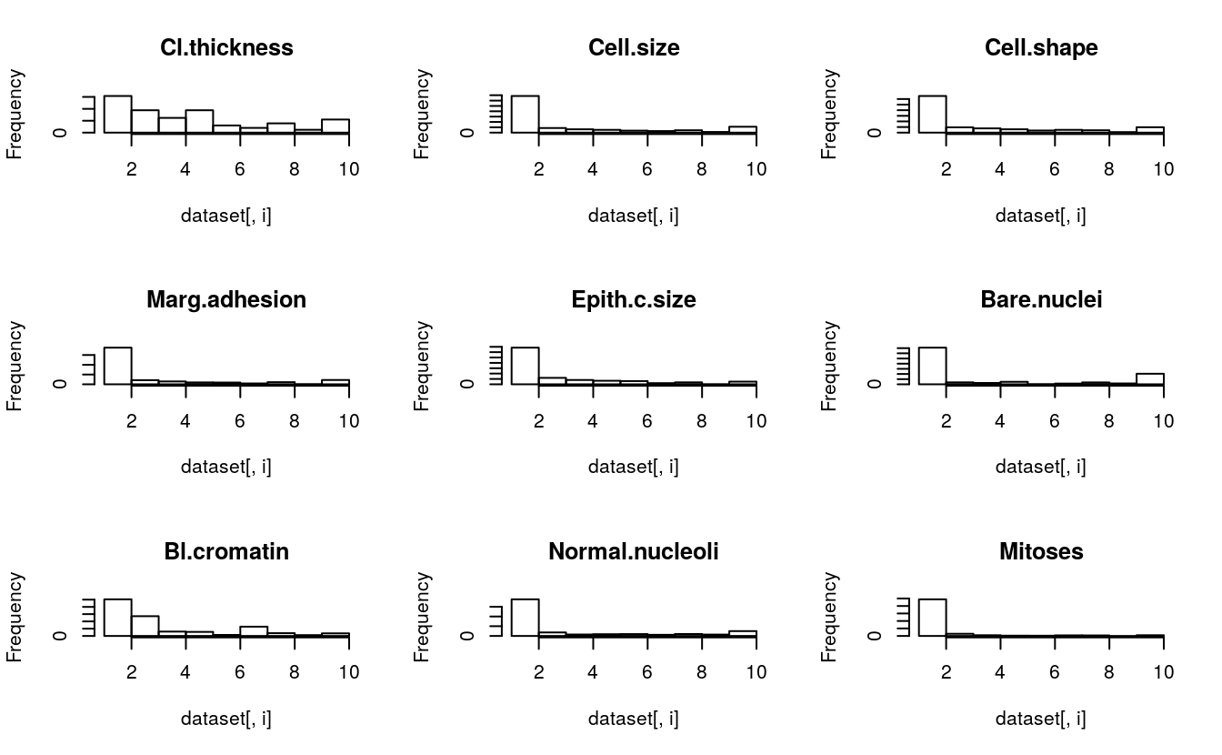
We can see that almost all of the distributions have an exponential or bimodal shape to them.
# density plot for each attribute
par(mfrow=c(3,3))
complete_cases <- complete.cases(dataset)
for(i in 1:9) {
    plot(density(dataset[complete_cases,i]), main=names(dataset)[i])
}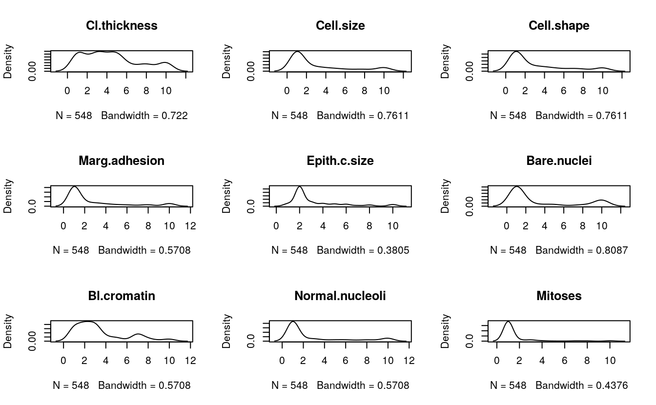
These plots add more support to our initial ideas. We can see bimodal distributions (two bumps) and exponential-looking distributions.
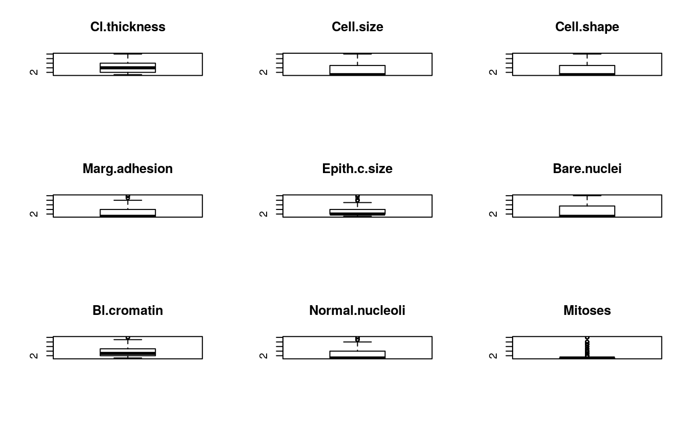
# boxplots for each attribute
par(mfrow=c(3,3))
for(i in 1:9) {
    boxplot(dataset[,i], main=names(dataset)[i])
}
21.7 Multimodal visualization
# scatter plot matrix
jittered_x <- sapply(dataset[,1:9], jitter)
pairs(jittered_x, names(dataset[,1:9]), col=dataset$Class)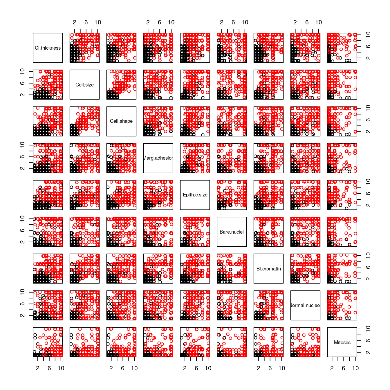
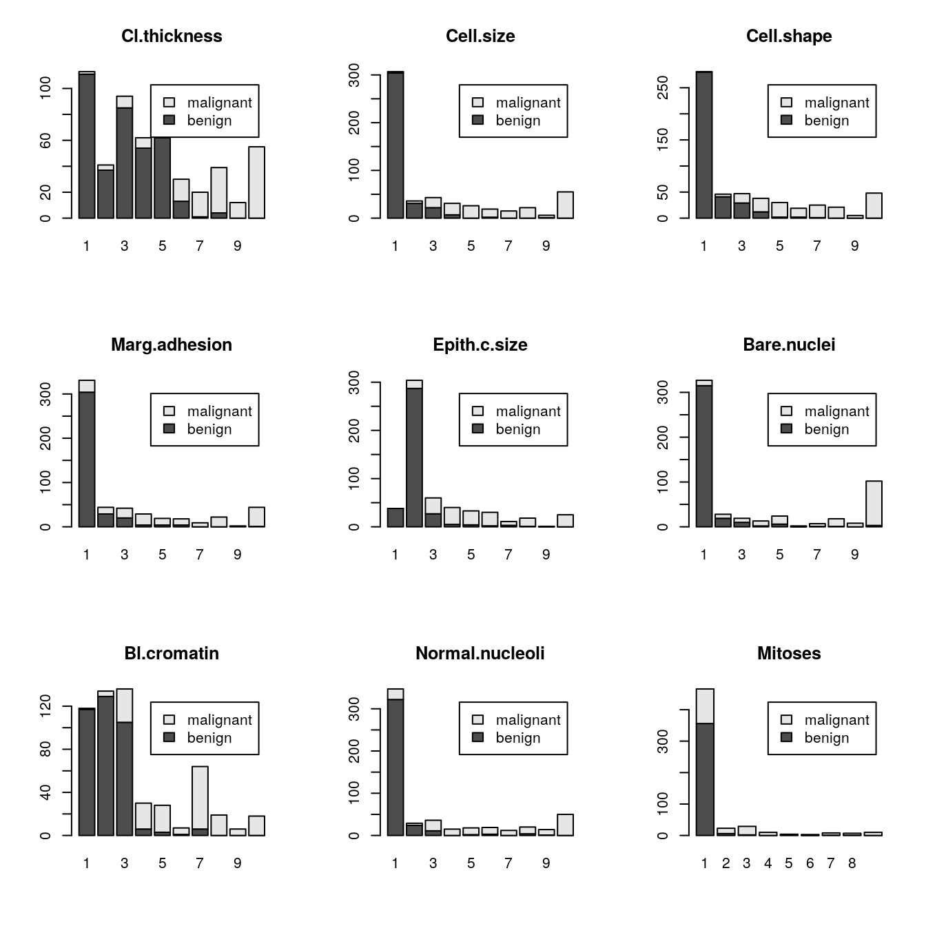
We can see that the black (benign) a part to be clustered around the bottom-right corner (smaller values) and red (malignant) are all over the place.
# bar plots of each variable by class
par(mfrow=c(3,3))
for(i in 1:9) {
    barplot(table(dataset$Class,dataset[,i]), main=names(dataset)[i],
            legend.text=unique(dataset$Class))
}
21.8 Algorithms Evaluation
Linear Algorithms: Logistic Regression (LG), Linear Discriminate Analysis (LDA) and Regularized Logistic Regression (GLMNET).
Nonlinear Algorithms: k-Nearest Neighbors (KNN), Classification and Regression Trees (CART), Naive Bayes (NB) and Support Vector Machines with Radial Basis Functions (SVM).
For simplicity, we will use Accuracy and Kappa metrics. Given that it is a medical test, we could have gone with the Area Under ROC Curve (AUC) and looked at the sensitivity and specificity to select the best algorithms.
# 10-fold cross-validation with 3 repeats
trainControl <- trainControl(method = "repeatedcv", number=10, repeats=3)
metric <- "Accuracy"
tic()
# LG
set.seed(7)
fit.glm <- train(Class~., data=dataset, method="glm", metric=metric,
                 trControl=trainControl, na.action=na.omit)
# LDA
set.seed(7)
fit.lda <- train(Class~., data=dataset, method="lda", metric=metric,
                 trControl=trainControl, na.action=na.omit)
# GLMNET
set.seed(7)
fit.glmnet <- train(Class~., data=dataset, method="glmnet", metric=metric,
                    trControl=trainControl, na.action=na.omit)
# KNN
set.seed(7)
fit.knn <- train(Class~., data=dataset, method="knn", metric=metric,
                 trControl=trainControl, na.action=na.omit)
# CART
set.seed(7)
fit.cart <- train(Class~., data=dataset, method="rpart", metric=metric,
                  trControl=trainControl, na.action=na.omit)
# Naive Bayes
set.seed(7)
fit.nb <- train(Class~., data=dataset, method="nb", metric=metric,
                trControl=trainControl, na.action=na.omit)
# SVM
set.seed(7)
fit.svm <- train(Class~., data=dataset, method="svmRadial", metric=metric,
                 trControl=trainControl, na.action=na.omit)

# Compare algorithms
results <- resamples(list(LG     = fit.glm,
                          LDA    = fit.lda,
                          GLMNET = fit.glmnet,
                          KNN    = fit.knn,
                          CART   = fit.cart,
                          NB     = fit.nb,
                          SVM    = fit.svm))
toc()
#> 14.162 sec elapsed
summary(results)
#>
#> Call:
#> summary.resamples(object = results)
#>
#> Models: LG, LDA, GLMNET, KNN, CART, NB, SVM
#> Number of resamples: 30
#>
#> Accuracy
#>         Min. 1st Qu. Median  Mean 3rd Qu. Max. NA's
#> LG     0.909   0.945  0.964 0.968   0.995    1    0
#> LDA    0.907   0.945  0.964 0.963   0.982    1    0
#> GLMNET 0.927   0.964  0.964 0.973   0.995    1    0
#> KNN    0.927   0.964  0.982 0.976   1.000    1    0
#> CART   0.833   0.927  0.945 0.943   0.964    1    0
#> NB     0.927   0.963  0.981 0.970   0.982    1    0
#> SVM    0.907   0.945  0.964 0.965   0.982    1    0
#>
#> Kappa
#>         Min. 1st Qu. Median  Mean 3rd Qu. Max. NA's
#> LG     0.806   0.880  0.921 0.930   0.990    1    0
#> LDA    0.786   0.880  0.918 0.917   0.959    1    0
#> GLMNET 0.843   0.918  0.922 0.940   0.990    1    0
#> KNN    0.843   0.920  0.959 0.947   1.000    1    0
#> CART   0.630   0.840  0.879 0.876   0.920    1    0
#> NB     0.835   0.918  0.959 0.934   0.960    1    0
#> SVM    0.804   0.883  0.922 0.926   0.960    1    0
dotplot(results)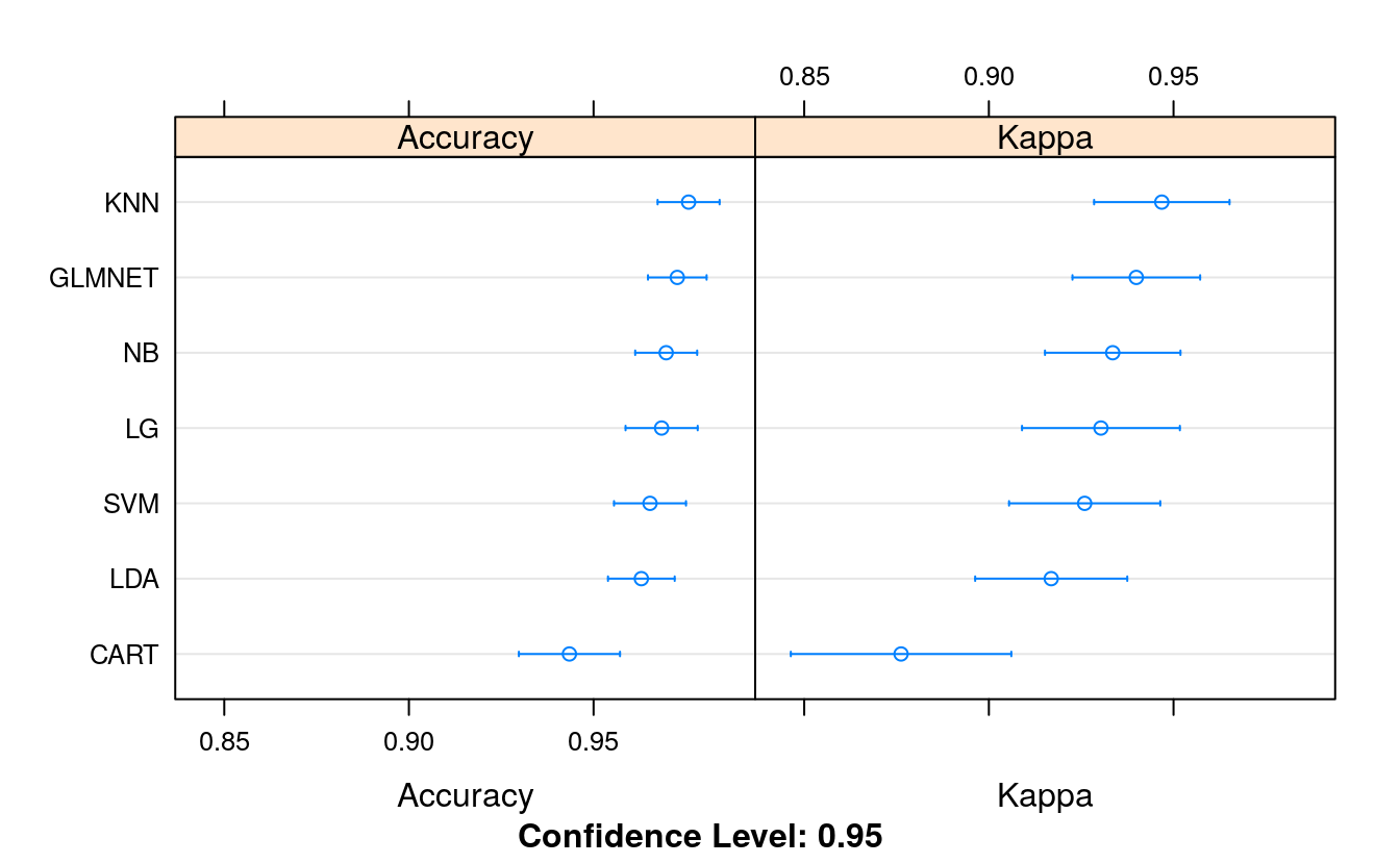
We can see good accuracy across the board. All algorithms have a mean accuracy above 90%, well above the baseline of 65% if we just predicted benign. The problem is learnable. We can see that KNN (97.08%) and logistic regression (NB was 96.2% and GLMNET was 96.4%) had the highest accuracy on the problem.
21.9 Data transform
We know we have some skewed distributions. There are transform methods that we can use to adjust and normalize these distributions. A favorite for positive input attributes (which we have in this case) is the Box-Cox transform.
# 10-fold cross-validation with 3 repeats
trainControl <- trainControl(method="repeatedcv", number=10, repeats=3)
metric <- "Accuracy"

# LG
set.seed(7)
fit.glm <- train(Class~., data=dataset, method="glm", metric=metric,
                 preProc=c("BoxCox"),
                 trControl=trainControl, na.action=na.omit)
# LDA
set.seed(7)
fit.lda <- train(Class~., data=dataset, method="lda", metric=metric,
                 preProc=c("BoxCox"),
                 trControl=trainControl, na.action=na.omit)
# GLMNET
set.seed(7)
fit.glmnet <- train(Class~., data=dataset, method="glmnet", metric=metric,
                    preProc=c("BoxCox"),
                    trControl=trainControl,
                    na.action=na.omit)
# KNN
set.seed(7)
fit.knn <- train(Class~., data=dataset, method="knn", metric=metric,
                 preProc=c("BoxCox"),
                 trControl=trainControl, na.action=na.omit)
# CART
set.seed(7)
fit.cart <- train(Class~., data=dataset, method="rpart", metric=metric,
                  preProc=c("BoxCox"),
                  trControl=trainControl,
                  na.action=na.omit)
# Naive Bayes
set.seed(7)
fit.nb <- train(Class~., data=dataset, method="nb", metric=metric,
                preProc=c("BoxCox"), trControl=trainControl, na.action=na.omit)
#> Warning in FUN(X[[i]], ...): Numerical 0 probability for all classes with
#> observation 1
#> Warning in FUN(X[[i]], ...): Numerical 0 probability for all classes with
#> observation 24
#> Warning in FUN(X[[i]], ...): Numerical 0 probability for all classes with
#> observation 28
#> Warning in FUN(X[[i]], ...): Numerical 0 probability for all classes with
#> observation 20
#> Warning in FUN(X[[i]], ...): Numerical 0 probability for all classes with
#> observation 11
#> Warning in FUN(X[[i]], ...): Numerical 0 probability for all classes with
#> observation 18
#> Warning in FUN(X[[i]], ...): Numerical 0 probability for all classes with
#> observation 54
#> Warning in FUN(X[[i]], ...): Numerical 0 probability for all classes with
#> observation 3
#> Warning in FUN(X[[i]], ...): Numerical 0 probability for all classes with
#> observation 23
#> Warning in FUN(X[[i]], ...): Numerical 0 probability for all classes with
#> observation 21
#> Warning in FUN(X[[i]], ...): Numerical 0 probability for all classes with
#> observation 27
#> Warning in FUN(X[[i]], ...): Numerical 0 probability for all classes with
#> observation 53
#> Warning in FUN(X[[i]], ...): Numerical 0 probability for all classes with
#> observation 12
#> Warning in FUN(X[[i]], ...): Numerical 0 probability for all classes with
#> observation 9
#> Warning in FUN(X[[i]], ...): Numerical 0 probability for all classes with
#> observation 2
#> Warning in FUN(X[[i]], ...): Numerical 0 probability for all classes with
#> observation 17
#> Warning in FUN(X[[i]], ...): Numerical 0 probability for all classes with
#> observation 9
#> Warning in FUN(X[[i]], ...): Numerical 0 probability for all classes with
#> observation 55
#> Warning in FUN(X[[i]], ...): Numerical 0 probability for all classes with
#> observation 23
#> Warning in FUN(X[[i]], ...): Numerical 0 probability for all classes with
#> observation 32
# SVM
set.seed(7)
fit.svm <- train(Class~., data=dataset, method="svmRadial", metric=metric,
                 preProc=c("BoxCox"),
                 trControl=trainControl, na.action=na.omit)

# Compare algorithms
transformResults <- resamples(list(LG     = fit.glm,
                                  LDA    = fit.lda,
                                  GLMNET = fit.glmnet,
                                  KNN    = fit.knn,
                                  CART   = fit.cart,
                                  NB     = fit.nb,
                                  SVM    = fit.svm))
summary(transformResults)
#>
#> Call:
#> summary.resamples(object = transformResults)
#>
#> Models: LG, LDA, GLMNET, KNN, CART, NB, SVM
#> Number of resamples: 30
#>
#> Accuracy
#>         Min. 1st Qu. Median  Mean 3rd Qu. Max. NA's
#> LG     0.909   0.963  0.982 0.973   0.996    1    0
#> LDA    0.927   0.964  0.981 0.974   0.982    1    0
#> GLMNET 0.944   0.964  0.982 0.980   1.000    1    0
#> KNN    0.909   0.964  0.981 0.976   0.982    1    0
#> CART   0.833   0.927  0.945 0.943   0.964    1    0
#> NB     0.927   0.964  0.982 0.978   1.000    1    0
#> SVM    0.927   0.964  0.982 0.980   1.000    1    0
#>
#> Kappa
#>         Min. 1st Qu. Median  Mean 3rd Qu. Max. NA's
#> LG     0.806   0.919  0.959 0.941   0.990    1    0
#> LDA    0.847   0.921  0.959 0.945   0.961    1    0
#> GLMNET 0.878   0.922  0.960 0.957   1.000    1    0
#> KNN    0.806   0.922  0.959 0.949   0.961    1    0
#> CART   0.630   0.840  0.879 0.876   0.920    1    0
#> NB     0.843   0.922  0.960 0.953   1.000    1    0
#> SVM    0.847   0.922  0.960 0.957   1.000    1    0
dotplot(transformResults)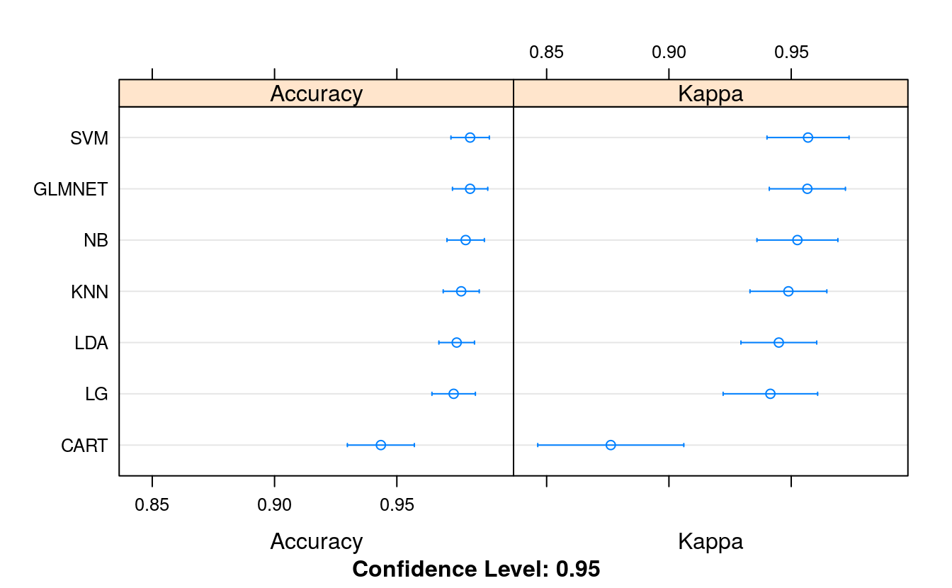
We can see that the accuracy of the previous best algorithm KNN was elevated to 97.14%. We have a new ranking, showing SVM with the most accurate mean accuracy at 97.20%.
21.10 Tuning SVM
# 10-fold cross-validation with 3 repeats
trainControl <- trainControl(method="repeatedcv", number=10, repeats=3)
metric <- "Accuracy"
set.seed(7)

grid <- expand.grid(.sigma = c(0.025, 0.05, 0.1, 0.15),
                    .C = seq(1, 10, by=1))

fit.svm <- train(Class~., data=dataset, method="svmRadial", metric=metric,
                 tuneGrid=grid,
                 preProc=c("BoxCox"), trControl=trainControl,
                 na.action=na.omit)
print(fit.svm)
#> Support Vector Machines with Radial Basis Function Kernel
#>
#> 560 samples
#>   9 predictor
#>   2 classes: 'benign', 'malignant'
#>
#> Pre-processing: Box-Cox transformation (9)
#> Resampling: Cross-Validated (10 fold, repeated 3 times)
#> Summary of sample sizes: 493, 492, 493, 493, 493, 494, ...
#> Resampling results across tuning parameters:
#>
#>   sigma  C   Accuracy  Kappa
#>   0.025   1  0.979     0.956
#>   0.025   2  0.979     0.954
#>   0.025   3  0.979     0.956
#>   0.025   4  0.977     0.950
#>   0.025   5  0.977     0.950
#>   0.025   6  0.978     0.951
#>   0.025   7  0.979     0.954
#>   0.025   8  0.979     0.956
#>   0.025   9  0.979     0.956
#>   0.025  10  0.979     0.956
#>   0.050   1  0.980     0.957
#>   0.050   2  0.980     0.957
#>   0.050   3  0.979     0.956
#>   0.050   4  0.980     0.957
#>   0.050   5  0.980     0.957
#>   0.050   6  0.980     0.957
#>   0.050   7  0.979     0.956
#>   0.050   8  0.979     0.954
#>   0.050   9  0.979     0.954
#>   0.050  10  0.979     0.954
#>   0.100   1  0.980     0.957
#>   0.100   2  0.980     0.957
#>   0.100   3  0.979     0.956
#>   0.100   4  0.978     0.953
#>   0.100   5  0.978     0.952
#>   0.100   6  0.975     0.946
#>   0.100   7  0.976     0.948
#>   0.100   8  0.976     0.948
#>   0.100   9  0.976     0.948
#>   0.100  10  0.975     0.946
#>   0.150   1  0.980     0.957
#>   0.150   2  0.978     0.953
#>   0.150   3  0.978     0.953
#>   0.150   4  0.976     0.949
#>   0.150   5  0.976     0.948
#>   0.150   6  0.975     0.946
#>   0.150   7  0.974     0.944
#>   0.150   8  0.972     0.939
#>   0.150   9  0.970     0.934
#>   0.150  10  0.968     0.930
#>
#> Accuracy was used to select the optimal model using the largest value.
#> The final values used for the model were sigma = 0.15 and C = 1.
plot(fit.svm)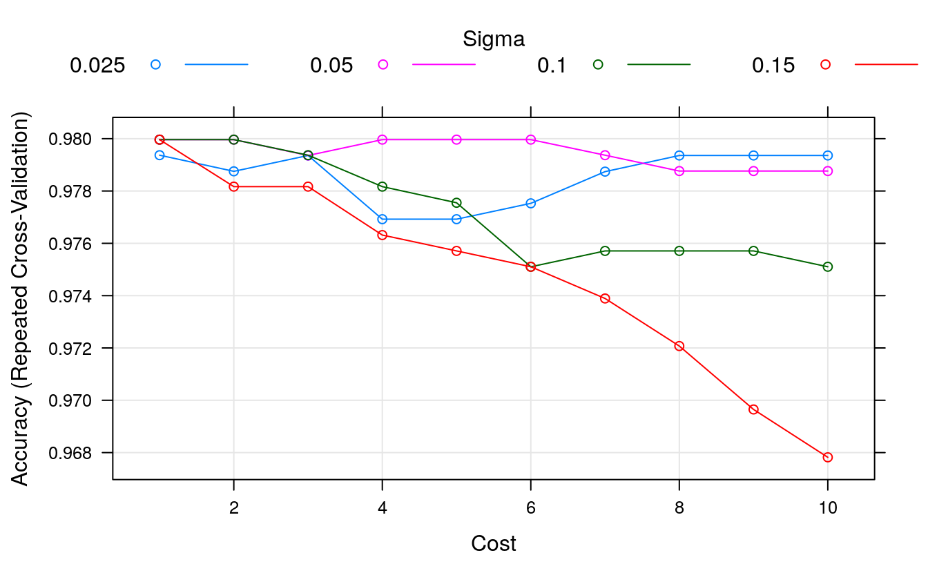
We can see that we have made very little difference to the results. The most accurate model had a score of 97.31% (the same as our previously rounded score of 97.20%) using a
sigma = 0.1andC = 1. We could tune further, but I don’t expect a payoff.
21.11 Tuning KNN
# 10-fold cross-validation with 3 repeats
trainControl <- trainControl(method="repeatedcv", number=10, repeats=3)
metric <- "Accuracy"
set.seed(7)

grid <- expand.grid(.k = seq(1,20, by=1))
fit.knn <- train(Class~., data=dataset, method="knn", metric=metric,
                 tuneGrid=grid,
                 preProc=c("BoxCox"), trControl=trainControl,
                 na.action=na.omit)
print(fit.knn)
#> k-Nearest Neighbors
#>
#> 560 samples
#>   9 predictor
#>   2 classes: 'benign', 'malignant'
#>
#> Pre-processing: Box-Cox transformation (9)
#> Resampling: Cross-Validated (10 fold, repeated 3 times)
#> Summary of sample sizes: 493, 492, 493, 493, 493, 494, ...
#> Resampling results across tuning parameters:
#>
#>   k   Accuracy  Kappa
#>    1  0.958     0.908
#>    2  0.960     0.912
#>    3  0.968     0.931
#>    4  0.970     0.935
#>    5  0.972     0.939
#>    6  0.973     0.942
#>    7  0.976     0.949
#>    8  0.975     0.946
#>    9  0.976     0.947
#>   10  0.976     0.949
#>   11  0.976     0.949
#>   12  0.976     0.947
#>   13  0.974     0.945
#>   14  0.975     0.946
#>   15  0.976     0.947
#>   16  0.975     0.946
#>   17  0.976     0.947
#>   18  0.976     0.947
#>   19  0.978     0.951
#>   20  0.977     0.950
#>
#> Accuracy was used to select the optimal model using the largest value.
#> The final value used for the model was k = 19.
plot(fit.knn)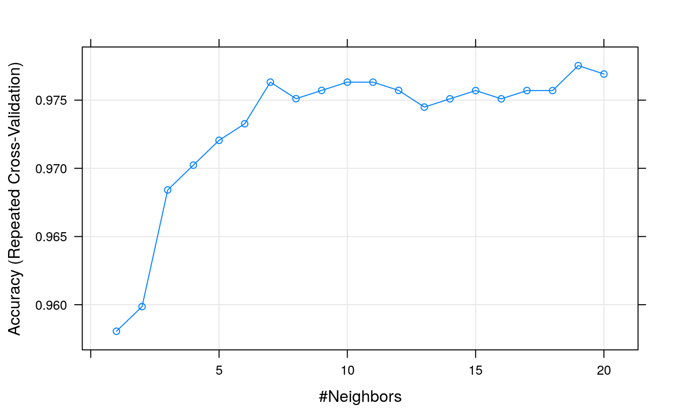
We can see again that tuning has made little difference, settling on a value of
k = 7with an accuracy of 97.19%. This is higher than the previous 97.14%, but very similar (or perhaps identical!) to the result achieved by the tuned SVM.
21.12 Ensemble
# 10-fold cross-validation with 3 repeats
trainControl <- trainControl(method="repeatedcv", number=10, repeats=3)
metric <- "Accuracy"

# Bagged CART
set.seed(7)
fit.treebag <- train(Class~., data=dataset, method="treebag",
                     metric=metric,
                     trControl=trainControl, na.action=na.omit)

# Random Forest
set.seed(7)
fit.rf <- train(Class~., data=dataset, method="rf",
                metric=metric, preProc=c("BoxCox"),
                trControl=trainControl, na.action=na.omit)

# Stochastic Gradient Boosting
set.seed(7)
fit.gbm <- train(Class~., data=dataset, method="gbm",
                 metric=metric, preProc=c("BoxCox"),
                 trControl=trainControl, verbose=FALSE, na.action=na.omit)

# C5.0
set.seed(7)
fit.c50 <- train(Class~., data=dataset, method="C5.0",
                 metric=metric, preProc=c("BoxCox"),
                 trControl=trainControl, na.action=na.omit)

# Compare results
ensembleResults <- resamples(list(BAG = fit.treebag,
                                  RF  = fit.rf,
                                  GBM = fit.gbm,
                                  C50 = fit.c50))
summary(ensembleResults)
#>
#> Call:
#> summary.resamples(object = ensembleResults)
#>
#> Models: BAG, RF, GBM, C50
#> Number of resamples: 30
#>
#> Accuracy
#>      Min. 1st Qu. Median  Mean 3rd Qu. Max. NA's
#> BAG 0.907   0.963  0.982 0.973   0.982    1    0
#> RF  0.926   0.981  0.982 0.979   0.995    1    0
#> GBM 0.929   0.963  0.981 0.973   0.995    1    0
#> C50 0.907   0.964  0.982 0.972   0.982    1    0
#>
#> Kappa
#>      Min. 1st Qu. Median  Mean 3rd Qu. Max. NA's
#> BAG 0.804   0.920  0.959 0.942    0.96    1    0
#> RF  0.841   0.959  0.960 0.955    0.99    1    0
#> GBM 0.844   0.919  0.959 0.941    0.99    1    0
#> C50 0.795   0.918  0.959 0.939    0.96    1    0
dotplot(ensembleResults)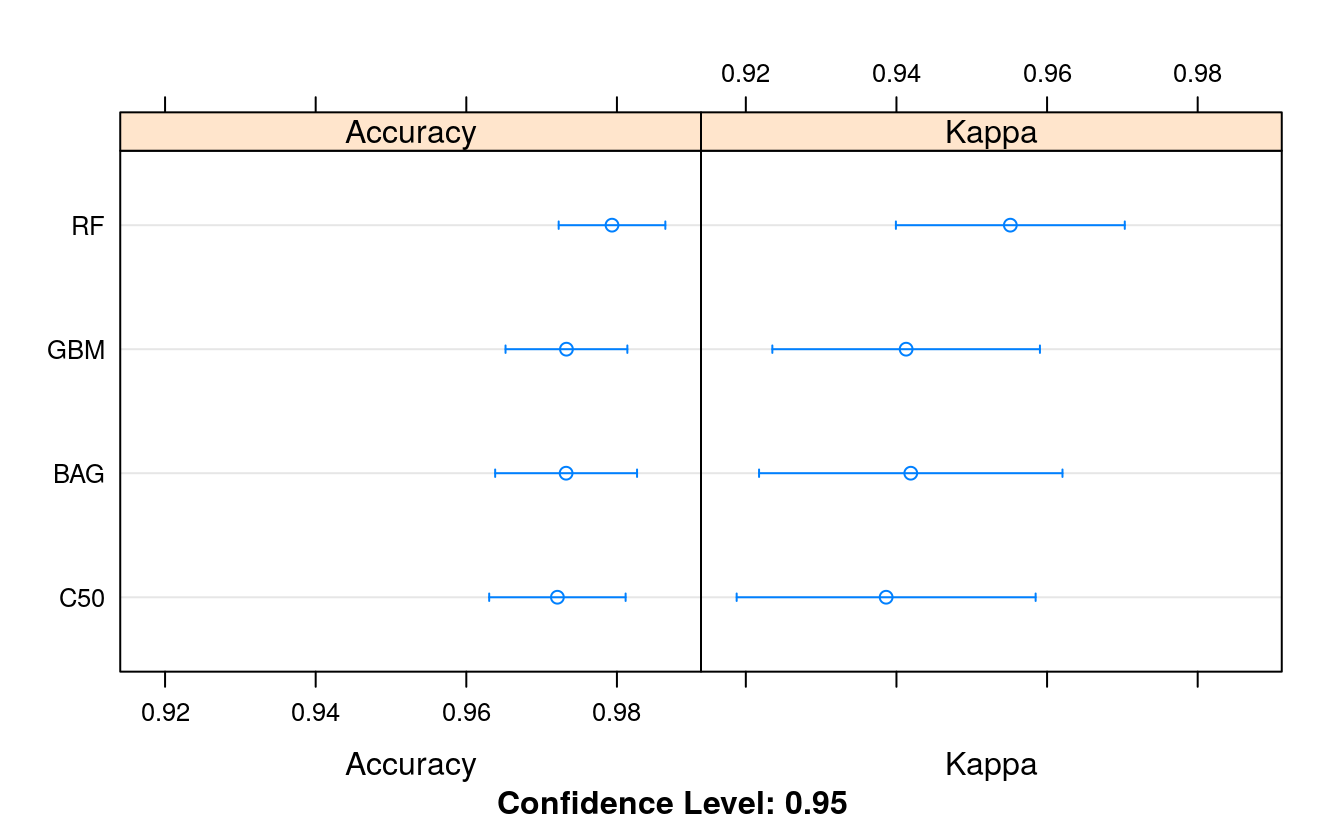
We see that Random Forest was the most accurate with a score of 97.26%. Very similar to our tuned models above. We could spend time tuning the parameters of Random Forest (e.g. increasing the number of trees) and the other ensemble methods, but I don’t expect to see better accuracy scores other than random statistical fluctuations.
21.13 Finalize model
We now need to finalize the model, which really means choose which model we would like to use. For simplicity I would probably select the KNN method, at the expense of the memory required to store the training dataset. SVM would be a good choice to trade-off space and time complexity. I probably would not select the Random Forest algorithm given the complexity of the model. It seems overkill for this dataset, lots of trees with little benefit in Accuracy.
Let’s go with the KNN algorithm. This is really simple, as we do not need to store a model. We do need to capture the parameters of the Box-Cox transform though. And we also need to prepare the data by removing the unused Id attribute and converting all of the inputs to numeric format.
The implementation of KNN (knn3()) belongs to the caret package and does not support missing values. We will have to remove the rows with missing values from the training dataset as well as the validation dataset. The code below shows the preparation of the pre-processing parameters using the training dataset.
# prepare parameters for data transform
set.seed(7)

datasetNoMissing <- dataset[complete.cases(dataset),]
x <- datasetNoMissing[,1:9]

# transform
preprocessParams <- preProcess(x, method=c("BoxCox"))
x <- predict(preprocessParams, x)
21.14 Prepare the validation set
Next we need to prepare the validation dataset for making a prediction. We must:
- Remove the Id attribute.
- Remove those rows with missing data.
- Convert all input attributes to numeric.
- Apply the Box-Cox transform to the input attributes using parameters prepared on the training dataset.
# prepare the validation dataset
set.seed(7)

# remove id column
validation <- validation[,-1]

# remove missing values (not allowed in this implementation of knn)
validation <- validation[complete.cases(validation),]

# convert to numeric
for(i in 1:9) {
    validation[,i] <- as.numeric(as.character(validation[,i]))
}

# transform the validation dataset
validationX <- predict(preprocessParams, validation[,1:9])
# make predictions
set.seed(7)
# knn3Train(train, test, cl, k = 1, l = 0, prob = TRUE, use.all = TRUE)
# k: number of neighbours considered.
predictions <- knn3Train(x, validationX, datasetNoMissing$Class,
                         k = 9,
                         prob = FALSE)

# convert
confusionMatrix(as.factor(predictions), validation$Class)
#> Confusion Matrix and Statistics
#>
#>            Reference
#> Prediction  benign malignant
#>   benign        83         1
#>   malignant      4        47
#>
#>                Accuracy : 0.963
#>                  95% CI : (0.916, 0.988)
#>     No Information Rate : 0.644
#>     P-Value [Acc > NIR] : <2e-16
#>
#>                   Kappa : 0.92
#>
#>  Mcnemar's Test P-Value : 0.371
#>
#>             Sensitivity : 0.954
#>             Specificity : 0.979
#>          Pos Pred Value : 0.988
#>          Neg Pred Value : 0.922
#>              Prevalence : 0.644
#>          Detection Rate : 0.615
#>    Detection Prevalence : 0.622
#>       Balanced Accuracy : 0.967
#>
#>        'Positive' Class : benign
#>
We can see that the accuracy of the final model on the validation dataset is 99.26%. This is optimistic because there is only 136 rows, but it does show that we have an accurate standalone model that we could use on other unclassified data.