17 Comparing Classification algorithms
- Datasets:
iris - Algorithms: LDA, CART, KNN, SVM, RF
17.2 Workflow
- Load dataset
- Create train and test datasets, 80/20
- Inspect dataset
- Visualize features
- Set the train control to
- 10 cross-validations
- Metric: accuracy
- Train the models
- Compare accuracy of models
- Visual comparison
- Make predictions on
validationset
We will split the loaded dataset into two, \(80\%\) of which we will use to train our models and \(20\%\) that we will hold back as a validation dataset.
# create a list of 80% of the rows in the original dataset we can use for training
validationIndex <- createDataPartition(dataset$Species, p=0.80, list=FALSE)
# select 20% of the data for validation
validation <- dataset[-validationIndex,]

# use the remaining 80% of data to training and testing the models
dataset <- dataset[validationIndex,]

# dimensions of dataset
dim(dataset)
#> [1] 120   5
# list types for each attribute
sapply(dataset, class)
#> Sepal.Length  Sepal.Width Petal.Length  Petal.Width      Species
#>    "numeric"    "numeric"    "numeric"    "numeric"     "factor"
17.3 Peek at the dataset
# take a peek at the first 5 rows of the data
head(dataset)
#>   Sepal.Length Sepal.Width Petal.Length Petal.Width Species
#> 1          5.1         3.5          1.4         0.2  setosa
#> 2          4.9         3.0          1.4         0.2  setosa
#> 3          4.7         3.2          1.3         0.2  setosa
#> 4          4.6         3.1          1.5         0.2  setosa
#> 5          5.0         3.6          1.4         0.2  setosa
#> 6          5.4         3.9          1.7         0.4  setosa
library(dplyr)
#>
#> Attaching package: 'dplyr'
#> The following objects are masked from 'package:stats':
#>
#>     filter, lag
#> The following objects are masked from 'package:base':
#>
#>     intersect, setdiff, setequal, union

glimpse(dataset)
#> Rows: 120
#> Columns: 5
#> $ Sepal.Length <dbl> 5.1, 4.9, 4.7, 4.6, 5.0, 5.4, 4.6, 5.0, 4.4, 4.9, 5.4, 4…
#> $ Sepal.Width  <dbl> 3.5, 3.0, 3.2, 3.1, 3.6, 3.9, 3.4, 3.4, 2.9, 3.1, 3.7, 3…
#> $ Petal.Length <dbl> 1.4, 1.4, 1.3, 1.5, 1.4, 1.7, 1.4, 1.5, 1.4, 1.5, 1.5, 1…
#> $ Petal.Width  <dbl> 0.2, 0.2, 0.2, 0.2, 0.2, 0.4, 0.3, 0.2, 0.2, 0.1, 0.2, 0…
#> $ Species      <fct> setosa, setosa, setosa, setosa, setosa, setosa, setosa, …
library(skimr)
print(skim(dataset))
#> ── Data Summary ────────────────────────
#>                            Values
#> Name                       dataset
#> Number of rows             120
#> Number of columns          5
#> _______________________
#> Column type frequency:
#>   factor                   1
#>   numeric                  4
#> ________________________
#> Group variables            None
#>
#> ── Variable type: factor ───────────────────────────────────────────────────────
#>   skim_variable n_missing complete_rate ordered n_unique
#> 1 Species               0             1 FALSE          3
#>   top_counts
#> 1 set: 40, ver: 40, vir: 40
#>
#> ── Variable type: numeric ──────────────────────────────────────────────────────
#>   skim_variable n_missing complete_rate  mean    sd    p0   p25   p50   p75
#> 1 Sepal.Length          0             1  5.86 0.837   4.3  5.1   5.8   6.4
#> 2 Sepal.Width           0             1  3.06 0.437   2    2.8   3     3.32
#> 3 Petal.Length          0             1  3.76 1.78    1    1.58  4.35  5.1
#> 4 Petal.Width           0             1  1.20 0.759   0.1  0.3   1.3   1.8
#>    p100 hist
#> 1   7.9 ▆▇▇▅▂
#> 2   4.4 ▁▆▇▂▁
#> 3   6.9 ▇▁▆▇▂
#> 4   2.5 ▇▁▆▅▃
17.4 Levels of the class
# list the levels for the class
levels(dataset$Species)
#> [1] "setosa"     "versicolor" "virginica"
17.5 class distribution
# summarize the class distribution
percentage <- prop.table(table(dataset$Species)) * 100
cbind(freq=table(dataset$Species), percentage=percentage)
#>            freq percentage
#> setosa       40       33.3
#> versicolor   40       33.3
#> virginica    40       33.3
17.6 Visualize the dataset
# split input and output
x <- dataset[,1:4]
y <- dataset[,5]
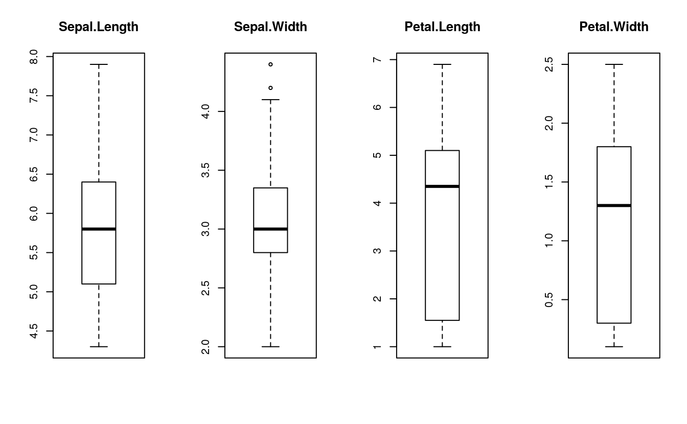
# boxplot for each attribute on one image
par(mfrow=c(1,4))
for(i in 1:4) {
    boxplot(x[,i], main=names(dataset)[i])
}
# barplot for class breakdown
plot(y)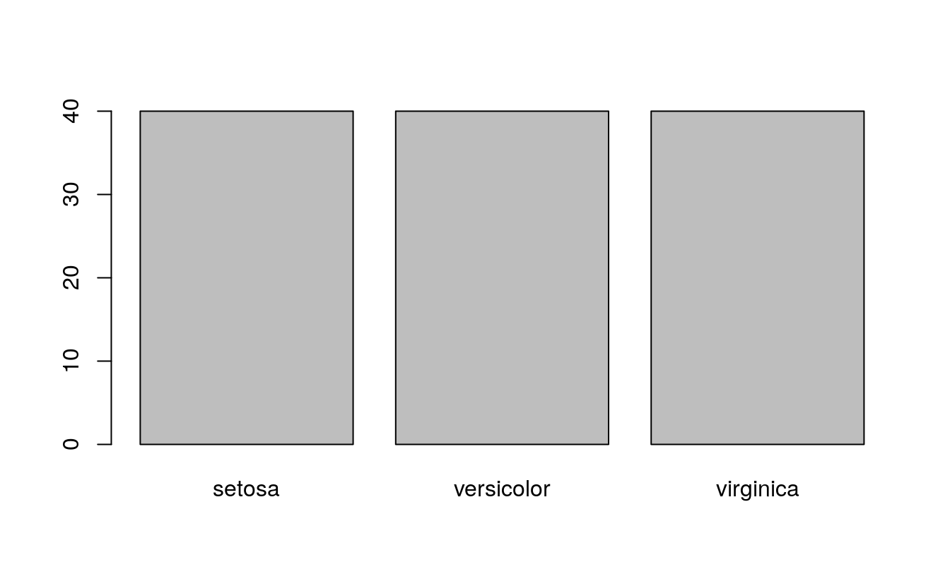
# scatter plot matrix
featurePlot(x=x, y=y, plot="ellipse")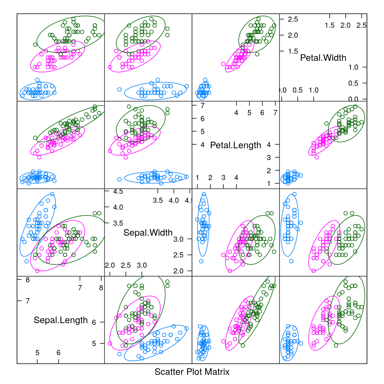
# box and whisker plots for each attribute
featurePlot(x=x, y=y, plot="box")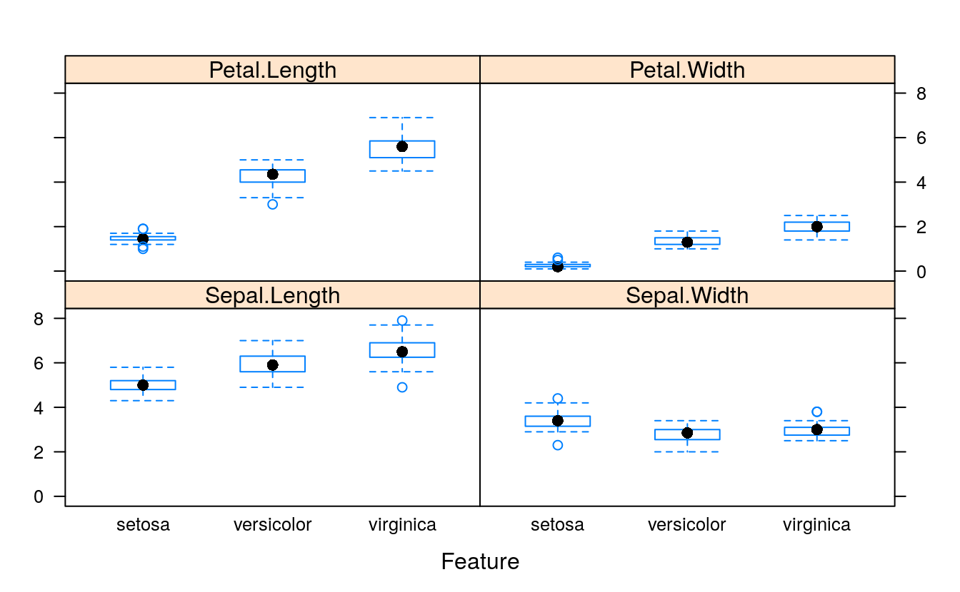
# density plots for each attribute by class value
scales <- list(x=list(relation="free"), y=list(relation="free"))
featurePlot(x=x, y=y, plot="density", scales=scales)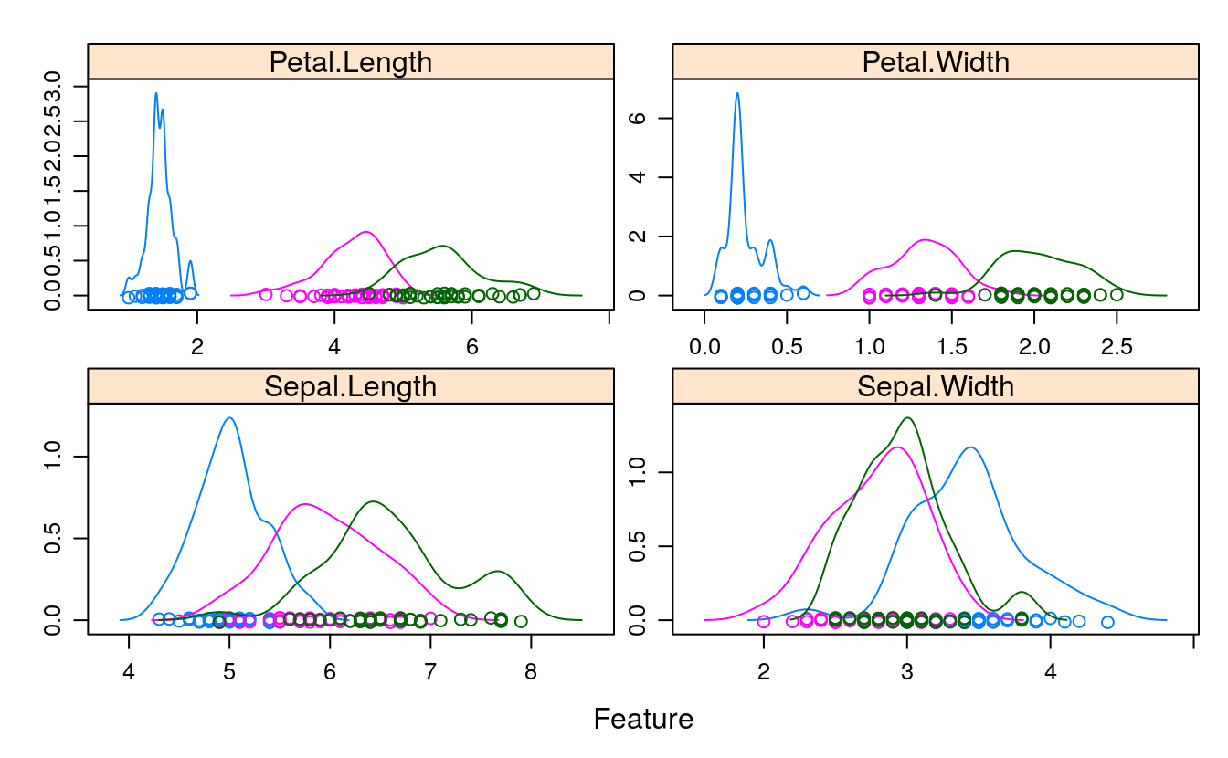
17.7 Evaluate algorithms
17.7.1 split and metrics
# Run algorithms using 10-fold cross-validation
trainControl <- trainControl(method="cv", number=10)
metric <- "Accuracy"
17.7.2 build models
# LDA
set.seed(7)
fit.lda <- train(Species~., data=dataset, method = "lda",
                 metric=metric, trControl=trainControl)
# CART
set.seed(7)
fit.cart <- train(Species~., data=dataset, method = "rpart",
                  metric=metric, trControl=trainControl)
# KNN
set.seed(7)
fit.knn <- train(Species~., data=dataset, method = "knn",
                 metric=metric, trControl=trainControl)
# SVM
set.seed(7)
fit.svm <- train(Species~., data=dataset, method = "svmRadial",
                 metric=metric, trControl=trainControl)
# Random Forest
set.seed(7)
fit.rf <- train(Species~., data=dataset, method = "rf",
                metric=metric, trControl=trainControl)
17.7.3 compare
#summarize accuracy of models
results <- resamples(list(lda  = fit.lda,
                          cart = fit.cart,
                          knn  = fit.knn,
                          svm  = fit.svm,
                          rf   = fit.rf))
summary(results)
#>
#> Call:
#> summary.resamples(object = results)
#>
#> Models: lda, cart, knn, svm, rf
#> Number of resamples: 10
#>
#> Accuracy
#>       Min. 1st Qu. Median  Mean 3rd Qu. Max. NA's
#> lda  0.917   1.000      1 0.992       1    1    0
#> cart 0.917   0.917      1 0.967       1    1    0
#> knn  0.917   0.938      1 0.975       1    1    0
#> svm  0.833   0.917      1 0.958       1    1    0
#> rf   0.917   0.917      1 0.967       1    1    0
#>
#> Kappa
#>       Min. 1st Qu. Median  Mean 3rd Qu. Max. NA's
#> lda  0.875   1.000      1 0.987       1    1    0
#> cart 0.875   0.875      1 0.950       1    1    0
#> knn  0.875   0.906      1 0.962       1    1    0
#> svm  0.750   0.875      1 0.937       1    1    0
#> rf   0.875   0.875      1 0.950       1    1    0
# compare accuracy of models
dotplot(results)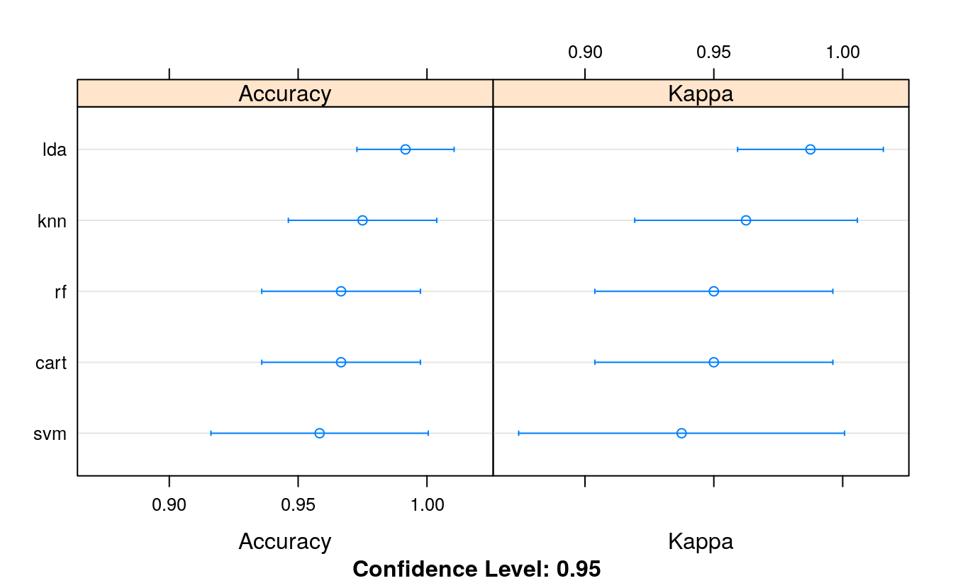
# summarize Best Model
print(fit.lda)
#> Linear Discriminant Analysis
#>
#> 120 samples
#>   4 predictor
#>   3 classes: 'setosa', 'versicolor', 'virginica'
#>
#> No pre-processing
#> Resampling: Cross-Validated (10 fold)
#> Summary of sample sizes: 108, 108, 108, 108, 108, 108, ...
#> Resampling results:
#>
#>   Accuracy  Kappa
#>   0.992     0.987
17.8 Make predictions
# estimate skill of LDA on the validation dataset
predictions <- predict(fit.lda, validation)
confusionMatrix(predictions, validation$Species)
#> Confusion Matrix and Statistics
#>
#>             Reference
#> Prediction   setosa versicolor virginica
#>   setosa         10          0         0
#>   versicolor      0          9         1
#>   virginica       0          1         9
#>
#> Overall Statistics
#>
#>                Accuracy : 0.933
#>                  95% CI : (0.779, 0.992)
#>     No Information Rate : 0.333
#>     P-Value [Acc > NIR] : 8.75e-12
#>
#>                   Kappa : 0.9
#>
#>  Mcnemar's Test P-Value : NA
#>
#> Statistics by Class:
#>
#>                      Class: setosa Class: versicolor Class: virginica
#> Sensitivity                  1.000             0.900            0.900
#> Specificity                  1.000             0.950            0.950
#> Pos Pred Value               1.000             0.900            0.900
#> Neg Pred Value               1.000             0.950            0.950
#> Prevalence                   0.333             0.333            0.333
#> Detection Rate               0.333             0.300            0.300
#> Detection Prevalence         0.333             0.333            0.333
#> Balanced Accuracy            1.000             0.925            0.925