35 Finding the factors of happiness
Dataset: World Happiness, happiness
35.1 Introduction
Source: http://enhancedatascience.com/2017/04/25/r-basics-linear-regression-with-r/ Data: https://www.kaggle.com/unsdsn/world-happiness
Linear regression is one of the basics of statistics and machine learning. Hence, it is a must-have to know how to perform a linear regression with R and how to interpret the results.
Linear regression algorithm will fit the best straight line that fits the data? To do so, it will minimise the squared distance between the points of the dataset and the fitted line.
For this tutorial, we will use the World Happiness report dataset from Kaggle. This report analyses the Happiness of each country according to several factors such as wealth, health, family life, … Our goal will be to find the most important factors of happiness. What a noble goal!
35.2 A quick exploration of the data
Before fitting any model, we need to know our data better. First, let’s import the data into R. Please download the dataset from Kaggle and put it in your working directory.
The code below imports the data as data.table and clean the column names (a lot of . were appearing in the original ones)
require(data.table)
#> Loading required package: data.table
data_happiness_dir <- file.path(data_raw_dir, "happiness")

Happiness_Data = data.table(read.csv(file.path(data_happiness_dir, '2016.csv')))
colnames(Happiness_Data) <- gsub('.','',colnames(Happiness_Data), fixed=T)
Now, let’s plot a Scatter Plot Matrix to get a grasp of how our variables are related one to another. To do so, the GGally package is great.
require(ggplot2)
#> Loading required package: ggplot2
require(GGally)
#> Loading required package: GGally
#> Registered S3 method overwritten by 'GGally':
#>   method from
#>   +.gg   ggplot2
ggpairs(Happiness_Data[,c(4,7:13), with=F], lower = list( continuous = "smooth"))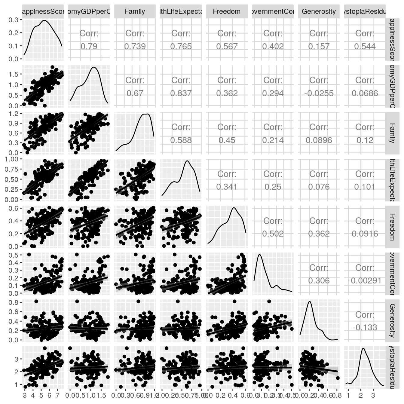
All the variables are positively correlated with the Happiness score. We can expect that most of the coefficients in the linear regression will be positive. However, the correlation between the variable is often more than 0.5, so we can expect that multicollinearity will appear in the regression.
In the data, we also have access to the Country where the score was computed. Even if it’s not useful for the regression, let’s plot the data on a map!
require('rworldmap')
#> Loading required package: rworldmap
#> Loading required package: sp
#> ### Welcome to rworldmap ###
#> For a short introduction type :   vignette('rworldmap')
library(reshape2)
#>
#> Attaching package: 'reshape2'
#> The following objects are masked from 'package:data.table':
#>
#>     dcast, melt

map.world <- map_data(map="world")

dataPlot<- melt(Happiness_Data, id.vars ='Country',
                measure.vars = colnames(Happiness_Data)[c(4,7:13)])

#Correcting names that are different
dataPlot[Country == 'United States', Country:='USA']
dataPlot[Country == 'United Kingdoms', Country:='UK']

##Rescaling each variable to have nice gradient
dataPlot[,value:=value/max(value), by=variable]
dataMap = data.table(merge(map.world, dataPlot,
                           by.x='region',
                           by.y='Country',
                           all.x=T))
dataMap = dataMap[order(order)]
dataMap = dataMap[order(order)][!is.na(variable)]
gg <- ggplot()
gg <- gg +
    geom_map(data=dataMap, map=dataMap,
             aes(map_id = region, x=long, y=lat, fill=value)) +
    # facet_wrap(~variable, scale='free')
    facet_wrap(~variable)
#> Warning: Ignoring unknown aesthetics: x, y
gg <- gg + scale_fill_gradient(low = "navy", high = "lightblue")
gg <- gg + coord_equal()
The code above is a classic code for a map. A few important points:
We reordered the point before plotting to avoid some artefacts. The merge is a right outer join, all the points of the map need to be kept. Otherwise, points will be missing which will mess up the map. Each variable is rescaled so that a facet_wrap can be used. Here, the absolute level of a variable is not of primary interest. This is the relative level of a variable between countries that we want to visualise.
gg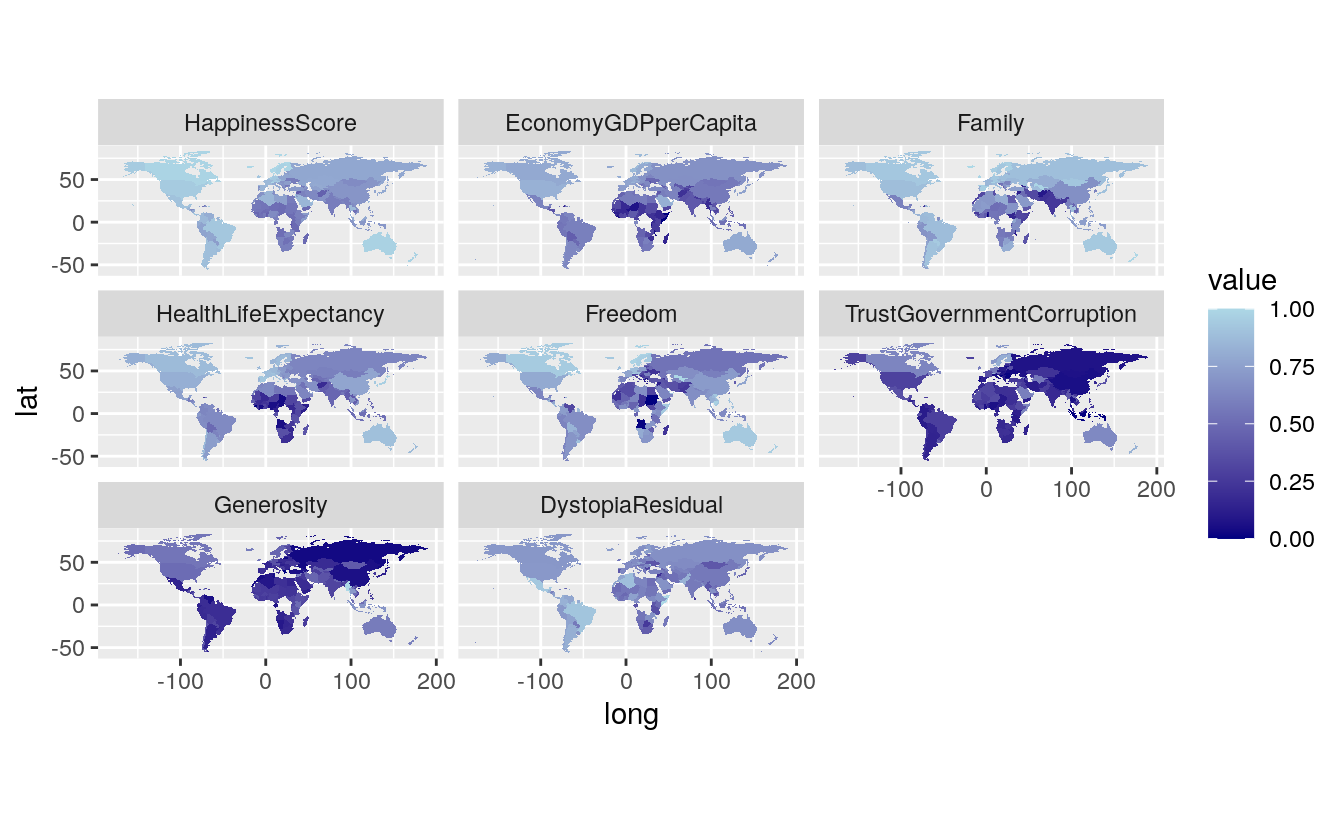
The distinction between North and South is quite visible. In addition to this, countries that have suffered from the crisis are also really visible.
35.3 Linear regression with R
Now that we have taken a look at our data, a first model can be fitted. The explanatory variables are the DGP per capita, the life expectancy, the level of freedom and the trust in the government.
##First model
model1 <- lm(HappinessScore ~ EconomyGDPperCapita + Family +
                 HealthLifeExpectancy + Freedom + TrustGovernmentCorruption,
             data=Happiness_Data)
35.4 Regression summary
The summary function provides a very easy way to assess a linear regression in R.
require(stargazer)
#> Loading required package: stargazer
#>
#> Please cite as:
#>  Hlavac, Marek (2018). stargazer: Well-Formatted Regression and Summary Statistics Tables.
#>  R package version 5.2.2. https://CRAN.R-project.org/package=stargazer

##Quick summary
sum1=summary(model1)
sum1
#>
#> Call:
#> lm(formula = HappinessScore ~ EconomyGDPperCapita + Family +
#>     HealthLifeExpectancy + Freedom + TrustGovernmentCorruption,
#>     data = Happiness_Data)
#>
#> Residuals:
#>     Min      1Q  Median      3Q     Max
#> -1.4833 -0.2817 -0.0277  0.3280  1.4615
#>
#> Coefficients:
#>                           Estimate Std. Error t value Pr(>|t|)
#> (Intercept)                  2.212      0.150   14.73  < 2e-16 ***
#> EconomyGDPperCapita          0.697      0.209    3.33   0.0011 **
#> Family                       1.234      0.229    5.39  2.6e-07 ***
#> HealthLifeExpectancy         1.462      0.343    4.26  3.5e-05 ***
#> Freedom                      1.559      0.373    4.18  5.0e-05 ***
#> TrustGovernmentCorruption    0.959      0.455    2.11   0.0365 *
#> ---
#> Signif. codes:  0 '***' 0.001 '**' 0.01 '*' 0.05 '.' 0.1 ' ' 1
#>
#> Residual standard error: 0.535 on 151 degrees of freedom
#> Multiple R-squared:  0.787,  Adjusted R-squared:  0.78
#> F-statistic:  112 on 5 and 151 DF,  p-value: <2e-16

stargazer(model1,type='text')
#>
#> =====================================================
#>                               Dependent variable:
#>                           ---------------------------
#>                                 HappinessScore
#> -----------------------------------------------------
#> EconomyGDPperCapita                0.697***
#>                                     (0.209)
#>
#> Family                             1.230***
#>                                     (0.229)
#>
#> HealthLifeExpectancy               1.460***
#>                                     (0.343)
#>
#> Freedom                            1.560***
#>                                     (0.373)
#>
#> TrustGovernmentCorruption           0.959**
#>                                     (0.455)
#>
#> Constant                           2.210***
#>                                     (0.150)
#>
#> -----------------------------------------------------
#> Observations                          157
#> R2                                   0.787
#> Adjusted R2                          0.780
#> Residual Std. Error            0.535 (df = 151)
#> F Statistic                112.000*** (df = 5; 151)
#> =====================================================
#> Note:                     *p<0.1; **p<0.05; ***p<0.01
A quick interpretation:
- All the coefficient are significative at a .05 threshold
- The overall model is also significative
- It explains 78.7% of Happiness in the dataset
- As expected all the relationship between the explanatory variables and the output variable are positives.
The model is doing well!
You can also easily get a given indicator of the model performance, such as R², the different coefficients or the p-value of the overall model.
##R²
sum1$r.squared*100
#> [1] 78.7
##Coefficients
sum1$coefficients
#>                           Estimate Std. Error t value Pr(>|t|)
#> (Intercept)                  2.212      0.150   14.73 5.20e-31
#> EconomyGDPperCapita          0.697      0.209    3.33 1.10e-03
#> Family                       1.234      0.229    5.39 2.62e-07
#> HealthLifeExpectancy         1.462      0.343    4.26 3.53e-05
#> Freedom                      1.559      0.373    4.18 5.01e-05
#> TrustGovernmentCorruption    0.959      0.455    2.11 3.65e-02
##p-value
df(sum1$fstatistic[1],sum1$fstatistic[2],sum1$fstatistic[3])
#>    value
#> 3.39e-49

##Confidence interval of the coefficient
confint(model1,level = 0.95)
#>                            2.5 % 97.5 %
#> (Intercept)               1.9152   2.51
#> EconomyGDPperCapita       0.2833   1.11
#> Family                    0.7821   1.69
#> HealthLifeExpectancy      0.7846   2.14
#> Freedom                   0.8212   2.30
#> TrustGovernmentCorruption 0.0609   1.86
confint(model1,level = 0.99)
#>                            0.5 % 99.5 %
#> (Intercept)                1.820   2.60
#> EconomyGDPperCapita        0.151   1.24
#> Family                     0.637   1.83
#> HealthLifeExpectancy       0.568   2.36
#> Freedom                    0.585   2.53
#> TrustGovernmentCorruption -0.227   2.14
confint(model1,level = 0.90)
#>                             5 % 95 %
#> (Intercept)               1.963 2.46
#> EconomyGDPperCapita       0.350 1.04
#> Family                    0.856 1.61
#> HealthLifeExpectancy      0.895 2.03
#> Freedom                   0.941 2.18
#> TrustGovernmentCorruption 0.207 1.71
35.5 Regression analysis
35.5.1 Residual analysis
Now that the regression has been done, the analysis and validity of the result can be analysed. Let’s begin with residuals and the assumption of normality and homoscedasticity.
# Visualisation of residuals
ggplot(model1, aes(model1$residuals)) +
    geom_histogram(bins=20, aes(y = ..density..)) +
    geom_density(color='blue', fill = 'blue', alpha = 0.2) +
    geom_vline(xintercept = mean(model1$residuals), color='red') +
    stat_function(fun=dnorm, color="red", size=1,
                  args = list(mean = mean(model1$residuals),
                            sd = sd(model1$residuals))) +
    xlab('residuals values')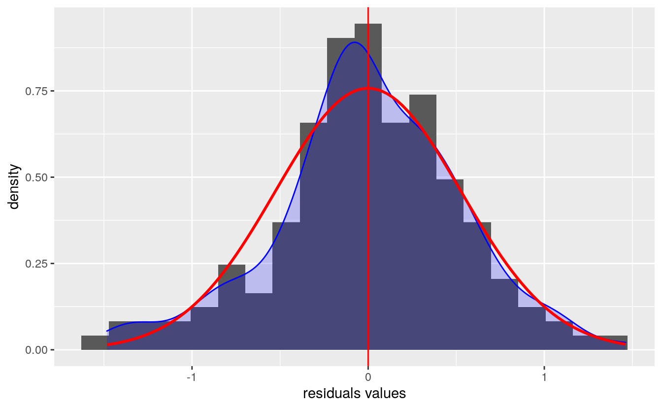
The residual versus fitted plot is used to see if the residuals behave the same for the different value of the output (i.e, they have the same variance and mean). The plot shows no strong evidence of heteroscedasticity.
ggplot(model1, aes(model1$fitted.values, model1$residuals)) +
    geom_point() +
    geom_hline(yintercept = c(1.96 * sd(model1$residuals),
                              - 1.96 * sd(model1$residuals)), color='red') +
    xlab('fitted value') +
    ylab('residuals values')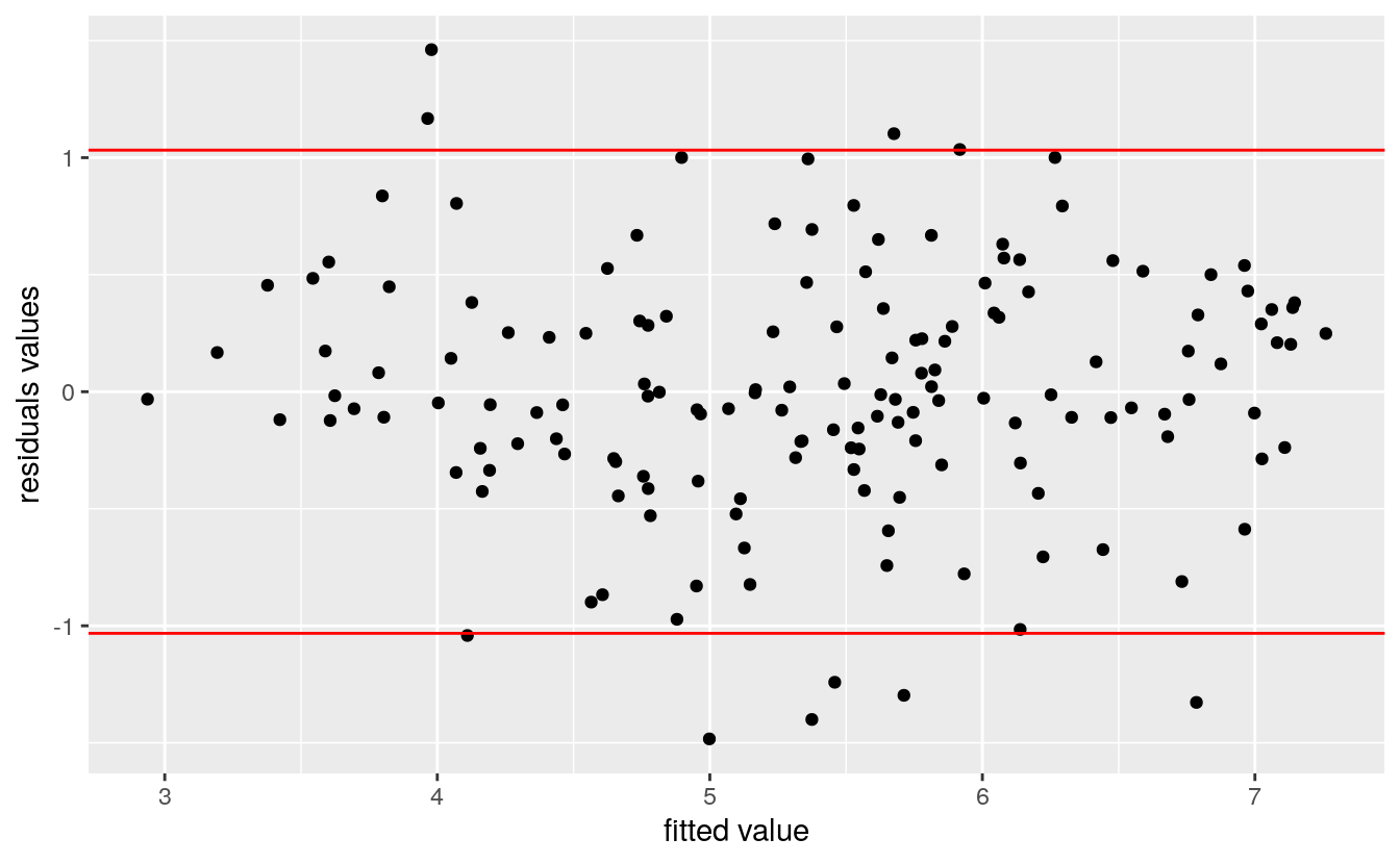
35.6 Analysis of colinearity
The colinearity can be assessed using VIF, the car package provides a function to compute it directly.
require('car')
#> Loading required package: car
#> Loading required package: carData
vif(model1)
#>       EconomyGDPperCapita                    Family      HealthLifeExpectancy
#>                      4.07                      2.03                      3.37
#>                   Freedom TrustGovernmentCorruption
#>                      1.61                      1.39
All the VIF are less than 5, and hence there is no sign of colinearity.
35.7 What drives happiness
Now let’s compute standardised betas to see what really drives happiness.
##Standardized betas
std_betas = sum1$coefficients[-1,1] *
    data.table(model1$model)[, lapply(.SD, sd), .SDcols=2:6] /
    sd(model1$model$HappinessScore)

std_betas
#>    EconomyGDPperCapita Family HealthLifeExpectancy Freedom
#> 1:               0.252  0.288                0.294   0.199
#>    TrustGovernmentCorruption
#> 1:                    0.0933
Though the code above may seem complicated, it is just computing the standardised betas for all variables std_beta=beta*sd(x)/sd(y).
The top three coefficients are Health and Life expectancy, Family and GDP per Capita. Though money does not make happiness it is among the top three factors of Happiness!
Now you know how to perform a linear regression with R!