45.1 Introduction

Regression ANNs predict an output variable as a function of the inputs. The input features (independent variables) can be categorical or numeric types, however, for regression ANNs, we require a numeric dependent variable. If the output variable is a categorical variable (or binary) the ANN will function as a classifier (see next tutorial).

Source: http://uc-r.github.io/ann_regression

In this tutorial we introduce a neural network used for numeric predictions and cover:

• Replication requirements: What you’ll need to reproduce the analysis in this tutorial.
• Data Preparation: Preparing our data.
• 1st Regression ANN: Constructing a 1-hidden layer ANN with 1 neuron.
• Regression Hyperparameters: Tuning the model.
• Wrapping Up: Final comments and some exercises to test your skills.

45.2 Replication Requirements

We require the following packages for the analysis.

library(tidyverse)
#> ── Attaching packages ─────────────────────────────────────── tidyverse 1.3.0 ──
#> ✔ ggplot2 3.3.0     ✔ purrr   0.3.4
#> ✔ tibble  3.0.1     ✔ dplyr   0.8.5
#> ✔ tidyr   1.0.2     ✔ stringr 1.4.0
#> ✔ readr   1.3.1     ✔ forcats 0.5.0
#> ── Conflicts ────────────────────────────────────────── tidyverse_conflicts() ──
#> ✖ dplyr::filter() masks stats::filter()
#> ✖ dplyr::lag()    masks stats::lag()
library(neuralnet)
#> 
#> Attaching package: 'neuralnet'
#> The following object is masked from 'package:dplyr':
#> 
#>     compute
library(GGally)
#> Registered S3 method overwritten by 'GGally':
#>   method from   
#>   +.gg   ggplot2
#> 
#> Attaching package: 'GGally'
#> The following object is masked from 'package:dplyr':
#> 
#>     nasa

45.3 Data Preparation

Our regression ANN will use the Yacht Hydrodynamics data set from UCI’s Machine Learning Repository. The yacht data was provided by Dr. Roberto Lopez email. This data set contains data contains results from 308 full-scale experiments performed at the Delft Ship Hydromechanics Laboratory where they test 22 different hull forms. Their experiment tested the effect of variations in the hull geometry and the ship’s Froude number on the craft’s residuary resistance per unit weight of displacement.

To begin we download the data from UCI.

url <- 'http://archive.ics.uci.edu/ml/machine-learning-databases/00243/yacht_hydrodynamics.data'

Yacht_Data <- read_table(file = url,
                         col_names = c('LongPos_COB', 'Prismatic_Coeff',
                                       'Len_Disp_Ratio', 'Beam_Draut_Ratio', 
                                       'Length_Beam_Ratio','Froude_Num', 
                                       'Residuary_Resist')) %>%
  na.omit()
#> Parsed with column specification:
#> cols(
#>   LongPos_COB = col_double(),
#>   Prismatic_Coeff = col_double(),
#>   Len_Disp_Ratio = col_double(),
#>   Beam_Draut_Ratio = col_double(),
#>   Length_Beam_Ratio = col_double(),
#>   Froude_Num = col_double(),
#>   Residuary_Resist = col_double()
#> )

dplyr::glimpse(Yacht_Data)
#> Rows: 308
#> Columns: 7
#> $ LongPos_COB       <dbl> -2.3, -2.3, -2.3, -2.3, -2.3, -2.3, -2.3, -2.3, -2.…
#> $ Prismatic_Coeff   <dbl> 0.568, 0.568, 0.568, 0.568, 0.568, 0.568, 0.568, 0.…
#> $ Len_Disp_Ratio    <dbl> 4.78, 4.78, 4.78, 4.78, 4.78, 4.78, 4.78, 4.78, 4.7…
#> $ Beam_Draut_Ratio  <dbl> 3.99, 3.99, 3.99, 3.99, 3.99, 3.99, 3.99, 3.99, 3.9…
#> $ Length_Beam_Ratio <dbl> 3.17, 3.17, 3.17, 3.17, 3.17, 3.17, 3.17, 3.17, 3.1…
#> $ Froude_Num        <dbl> 0.125, 0.150, 0.175, 0.200, 0.225, 0.250, 0.275, 0.…
#> $ Residuary_Resist  <dbl> 0.11, 0.27, 0.47, 0.78, 1.18, 1.82, 2.61, 3.76, 4.9…

# save the dataset locally
write.csv(Yacht_Data, file = file.path(data_raw_dir, "yach_data.csv"))

Prior to any data analysis lets take a look at the data set.

ggpairs(Yacht_Data, title = "Scatterplot Matrix of the Features of the Yacht Data Set")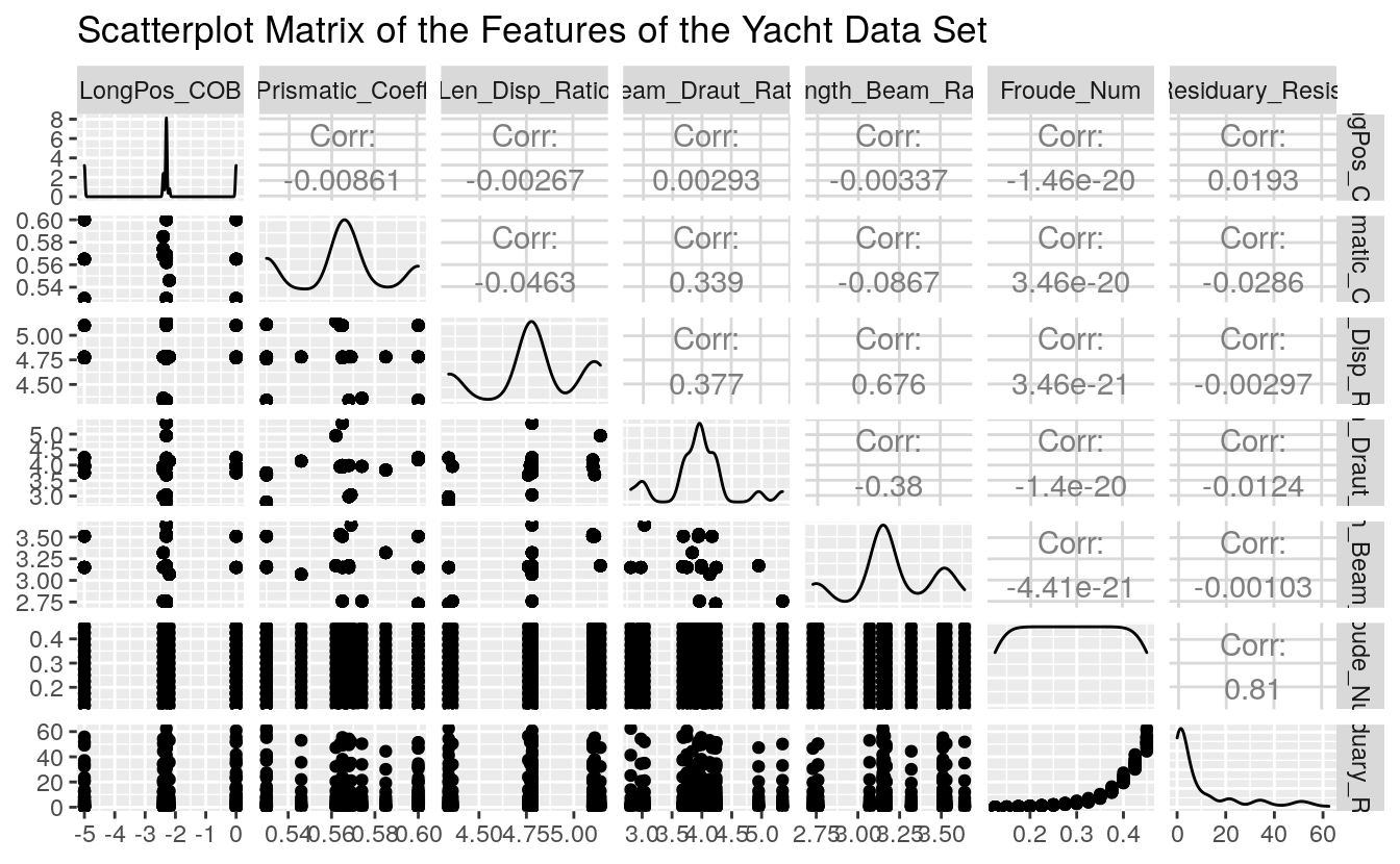

Here we see an excellent summary of the variation of each feature in our data set. Draw your attention to the bottom-most strip of scatter-plots. This shows the residuary resistance as a function of the other data set features (independent experimental values). The greatest variation appears with the Froude Number feature. It will be interesting to see how this pattern appears in the subsequent regression ANNs.

Prior to regression ANN construction we first must split the Yacht data set into test and training data sets. Before we split, first scale each feature to fall in the [0,1] interval.

# Scale the Data
scale01 <- function(x){
  (x - min(x)) / (max(x) - min(x))
}

Yacht_Data <- Yacht_Data %>%
  mutate_all(scale01)

# Split into test and train sets
set.seed(12345)
Yacht_Data_Train <- sample_frac(tbl = Yacht_Data, replace = FALSE, size = 0.80)
Yacht_Data_Test <- anti_join(Yacht_Data, Yacht_Data_Train)
#> Joining, by = c("LongPos_COB", "Prismatic_Coeff", "Len_Disp_Ratio", "Beam_Draut_Ratio", "Length_Beam_Ratio", "Froude_Num", "Residuary_Resist")

The scale01() function maps each data observation onto the [0,1] interval as called in the dplyr mutate_all() function. We then provided a seed for reproducible results and randomly extracted (without replacement) 80% of the observations to build the Yacht_Data_Train data set. Using dplyr’s anti_join() function we extracted all the observations not within the Yacht_Data_Train data set as our test data set in Yacht_Data_Test.

45.4 1st Regression ANN

To begin we construct a 1-hidden layer ANN with 1 neuron, the simplest of all neural networks.

set.seed(12321)
Yacht_NN1 <- neuralnet(Residuary_Resist ~ LongPos_COB + Prismatic_Coeff + 
                         Len_Disp_Ratio + Beam_Draut_Ratio + Length_Beam_Ratio +
                         Froude_Num, data = Yacht_Data_Train)

The Yacht_NN1 is a list containing all parameters of the regression ANN as well as the results of the neural network on the test data set. To view a diagram of the Yacht_NN1 use the plot() function.

plot(Yacht_NN1, rep = 'best')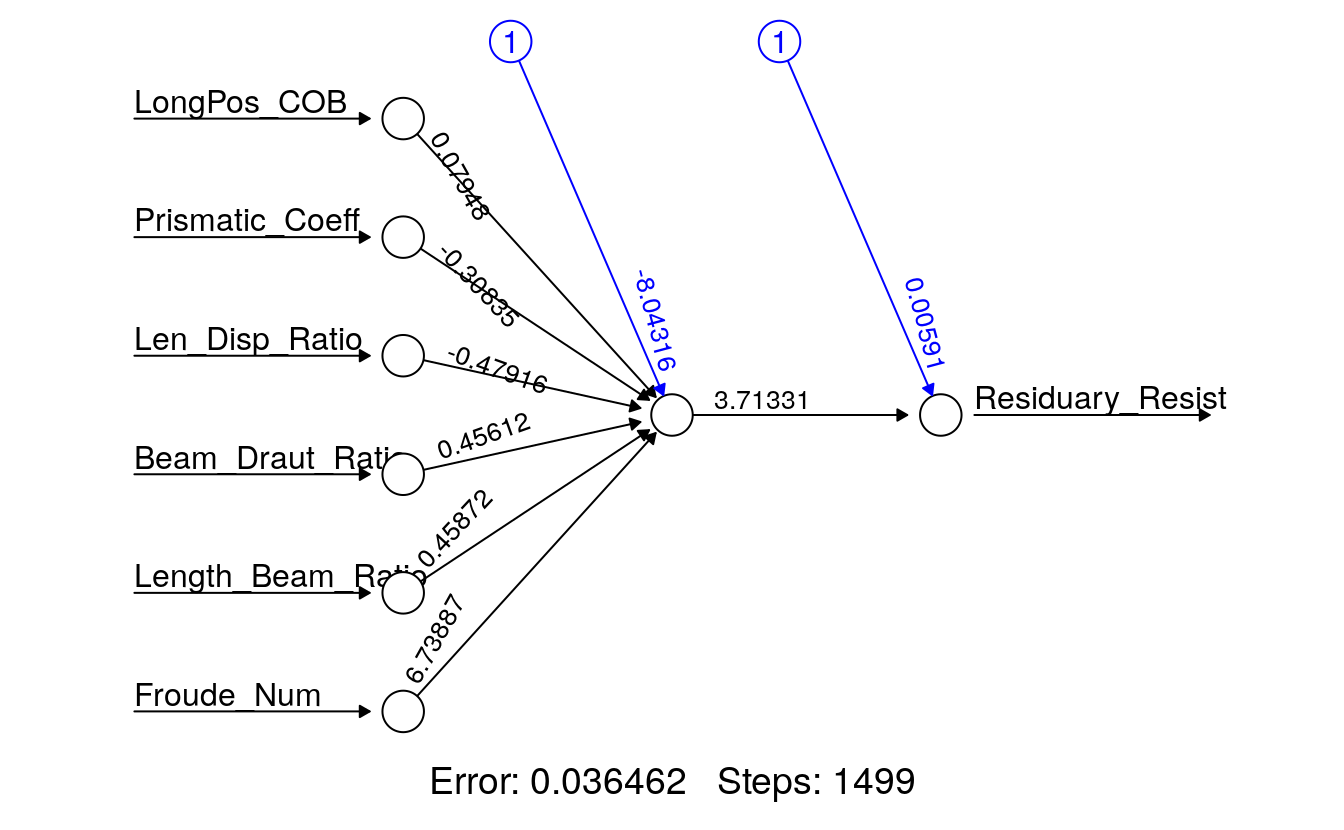

This plot shows the weights learned by the Yacht_NN1 neural network, and displays the number of iterations before convergence, as well as the SSE of the training data set. To manually compute the SSE you can use the following:

NN1_Train_SSE <- sum((Yacht_NN1$net.result - Yacht_Data_Train[, 7])^2)/2
paste("SSE: ", round(NN1_Train_SSE, 4))
#> [1] "SSE:  0.0365"
## [1] "SSE:  0.0361"

This SSE is the error associated with the training data set. A superior metric for estimating the generalization capability of the ANN would be the SSE of the test data set. Recall, the test data set contains observations not used to train the Yacht_NN1 ANN. To calculate the test error, we first must run our test observations through the Yacht_NN1 ANN. This is accomplished with the neuralnet package compute() function, which takes as its first input the desired neural network object created by the neuralnet() function, and the second argument the test data set feature (independent variable(s)) values.

Test_NN1_Output <- compute(Yacht_NN1, Yacht_Data_Test[, 1:6])$net.result
NN1_Test_SSE <- sum((Test_NN1_Output - Yacht_Data_Test[, 7])^2)/2
NN1_Test_SSE
#> [1] 0.0139
## [1] 0.008417631461

The compute() function outputs the response variable, in our case the Residuary_Resist, as estimated by the neural network. Once we have the ANN estimated response we can compute the test SSE. Comparing the test error of 0.0084 to the training error of 0.0361 we see that in our case our test error is smaller than our training error.

45.5 Regression Hyperparameters

We have constructed the most basic of regression ANNs without modifying any of the default hyperparameters associated with the neuralnet() function. We should try and improve the network by modifying its basic structure and hyperparameter modification. To begin we will add depth to the hidden layer of the network, then we will change the activation function from the logistic to the tangent hyperbolicus (tanh) to determine if these modifications can improve the test data set SSE. When using the tanh activation function, we first must rescale the data from \([0,1]\) to \([-1,1]\) using the rescale package. For the purposes of this exercise we will use the same random seed for reproducible results, generally this is not a best practice.

# 2-Hidden Layers, Layer-1 4-neurons, Layer-2, 1-neuron, logistic activation
# function
set.seed(12321)
Yacht_NN2 <- neuralnet(Residuary_Resist ~ LongPos_COB + Prismatic_Coeff + Len_Disp_Ratio + Beam_Draut_Ratio + Length_Beam_Ratio + Froude_Num, 
                       data = Yacht_Data_Train, 
                       hidden = c(4, 1), 
                       act.fct = "logistic")

## Training Error
NN2_Train_SSE <- sum((Yacht_NN2$net.result - Yacht_Data_Train[, 7])^2)/2

## Test Error
Test_NN2_Output <- compute(Yacht_NN2, Yacht_Data_Test[, 1:6])$net.result
NN2_Test_SSE <- sum((Test_NN2_Output - Yacht_Data_Test[, 7])^2)/2

# Rescale for tanh activation function
scale11 <- function(x) {
    (2 * ((x - min(x))/(max(x) - min(x)))) - 1
}
Yacht_Data_Train <- Yacht_Data_Train %>% mutate_all(scale11)
Yacht_Data_Test <- Yacht_Data_Test %>% mutate_all(scale11)

# 2-Hidden Layers, Layer-1 4-neurons, Layer-2, 1-neuron, tanh activation
# function
set.seed(12321)
Yacht_NN3 <- neuralnet(Residuary_Resist ~ LongPos_COB + Prismatic_Coeff + Len_Disp_Ratio + Beam_Draut_Ratio + Length_Beam_Ratio + Froude_Num, 
                       data = Yacht_Data_Train, 
                       hidden = c(4, 1), 
                       act.fct = "tanh")

## Training Error
NN3_Train_SSE <- sum((Yacht_NN3$net.result - Yacht_Data_Train[, 7])^2)/2

## Test Error
Test_NN3_Output <- compute(Yacht_NN3, Yacht_Data_Test[, 1:6])$net.result
NN3_Test_SSE <- sum((Test_NN3_Output - Yacht_Data_Test[, 7])^2)/2

# 1-Hidden Layer, 1-neuron, tanh activation function
set.seed(12321)
Yacht_NN4 <- neuralnet(Residuary_Resist ~ LongPos_COB + Prismatic_Coeff + Len_Disp_Ratio + Beam_Draut_Ratio + Length_Beam_Ratio + Froude_Num, 
                       data = Yacht_Data_Train, 
                       act.fct = "tanh")

## Training Error
NN4_Train_SSE <- sum((Yacht_NN4$net.result - Yacht_Data_Train[, 7])^2)/2

## Test Error
Test_NN4_Output <- compute(Yacht_NN4, Yacht_Data_Test[, 1:6])$net.result
NN4_Test_SSE <- sum((Test_NN4_Output - Yacht_Data_Test[, 7])^2)/2

# Bar plot of results
Regression_NN_Errors <- tibble(Network = rep(c("NN1", "NN2", "NN3", "NN4"), each = 2), 
                               DataSet = rep(c("Train", "Test"), time = 4), 
                               SSE = c(NN1_Train_SSE, NN1_Test_SSE, 
                                       NN2_Train_SSE, NN2_Test_SSE, 
                                       NN3_Train_SSE, NN3_Test_SSE, 
                                       NN4_Train_SSE, NN4_Test_SSE))

Regression_NN_Errors %>% 
  ggplot(aes(Network, SSE, fill = DataSet)) + 
  geom_col(position = "dodge") + 
  ggtitle("Regression ANN's SSE")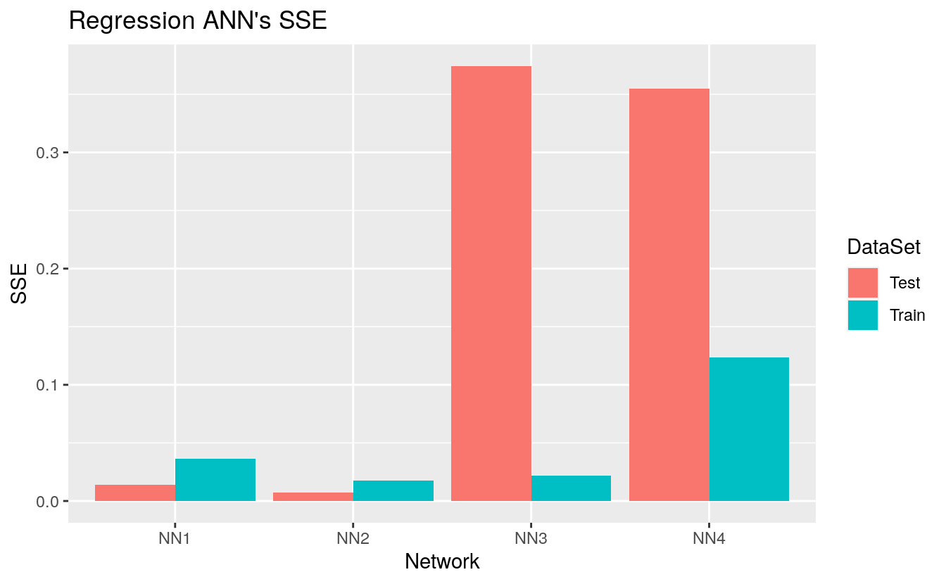

As evident from the plot, we see that the best regression ANN we found was Yacht_NN2 with a training and test SSE of 0.0188 and 0.0057. We make this determination by the value of the training and test SSEs only. Yacht_NN2’s structure is presented here:

plot(Yacht_NN2, rep = "best")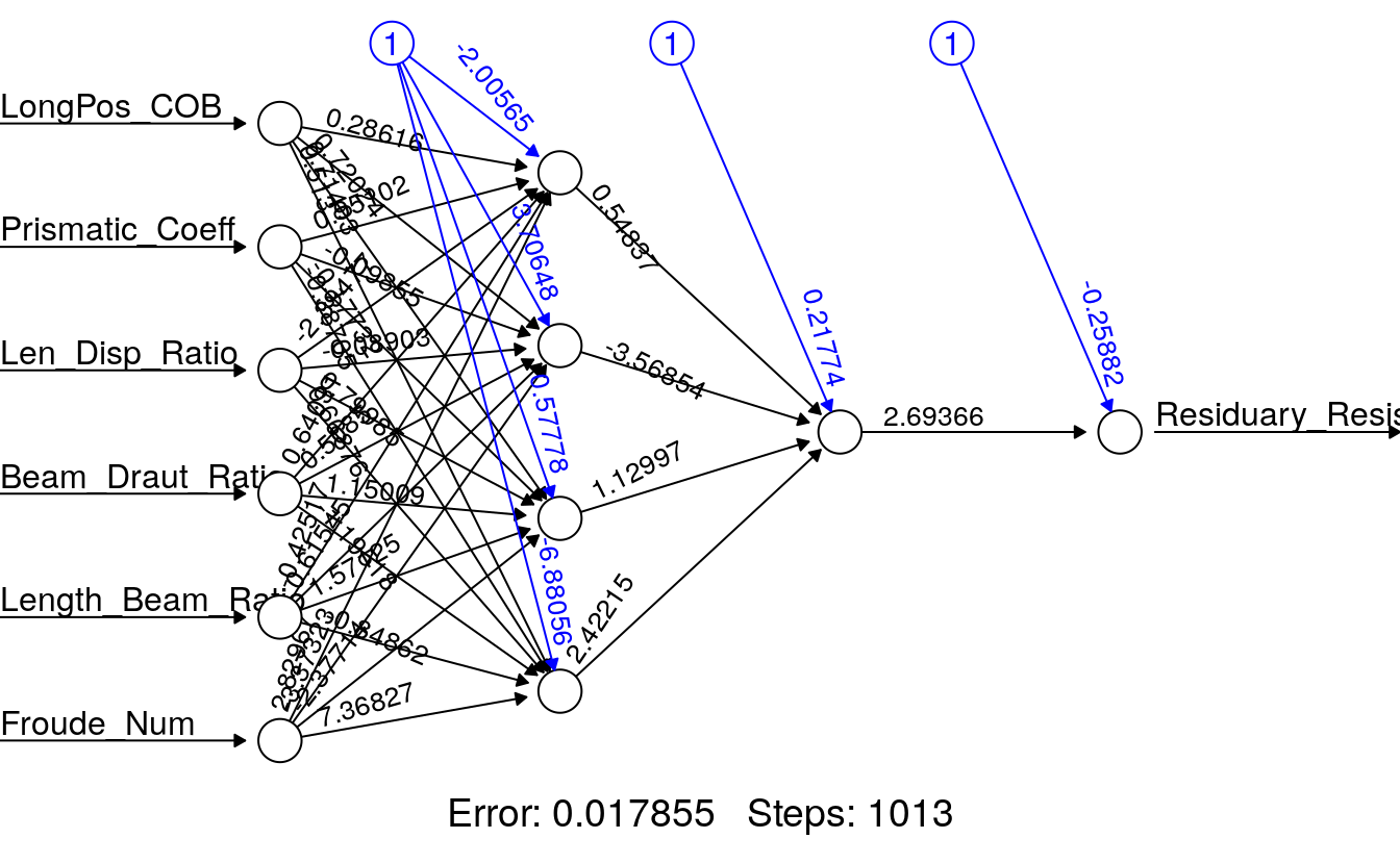

set.seed(12321)
Yacht_NN2 <- neuralnet(Residuary_Resist ~ LongPos_COB + Prismatic_Coeff + Len_Disp_Ratio + Beam_Draut_Ratio + Length_Beam_Ratio + Froude_Num, 
                       data = Yacht_Data_Train, 
                       hidden = c(4, 1), 
                       act.fct = "logistic", 
                       rep = 10)

plot(Yacht_NN2, rep = "best")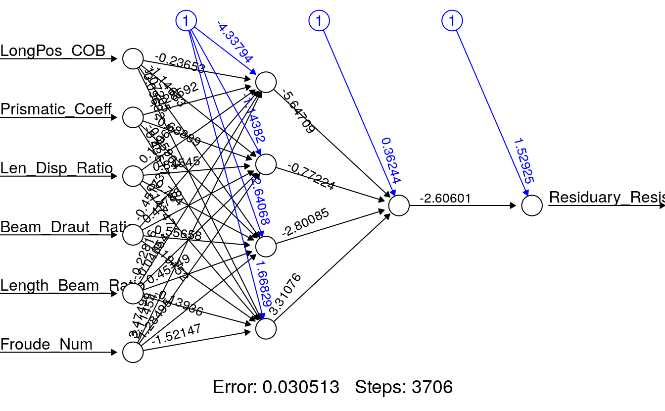

By setting the same seed, prior to running the 10 repetitions of ANNs, we force the software to reproduce the exact same Yacht_NN2 ANN for the first replication. The subsequent 9 generated ANNs, use a different random set of starting weights. Comparing the ‘best’ of the 10 repetitions, to the Yacht_NN2, we observe a decrease in training set error indicating we have a superior set of weights.

45.6 Wrapping Up

We have briefly covered regression ANNs in this tutorial. In the next tutorial we will cover classification ANNs. The neuralnet package used in this tutorial is one of many tools available for ANN implementation in R. Others include:

• nnet
• autoencoder
• caret
• RSNNS
• h2o

Before you move on to the next tutorial, test your new knowledge on the exercises that follow.

1. Why do we split the yacht data into a training and test data sets?

2. Re-load the Yacht Data from the UCI Machine learning repository yacht data without scaling. Run any regression ANN. What happens? Why do you think this happens?

3. After completing exercise question 1, re-scale the yacht data. Perform a simple linear regression fitting Residuary_Resist as a function of all other features. Now run a regression neural network (see 1st Regression ANN section). Plot the regression ANN and compare the weights on the features in the ANN to the p-values for the regressors.

4. Build your own regression ANN using the scaled yacht data modifying one hyperparameter. Use ?neuralnet to see the function options. Plot your ANN.