31 Linear Regression with ISLR
Dataset: Advertising.csv
Videos, slides:
Data:
code:
- http://subasish.github.io/pages/ISLwithR/
- http://math480-s15-zarringhalam.wikispaces.umb.edu/R+Code
- https://github.com/yahwes/ISLR
- https://www.tau.ac.il/~saharon/IntroStatLearn.html
- https://www.waxworksmath.com/Authors/G_M/James/WWW/chapter_3.html
- https://github.com/asadoughi/stat-learning
plots:
library(readr)

advertising <- read_csv(file.path(data_raw_dir, "Advertising.csv"))
#> Warning: Missing column names filled in: 'X1' [1]
#> Parsed with column specification:
#> cols(
#>   X1 = col_double(),
#>   TV = col_double(),
#>   radio = col_double(),
#>   newspaper = col_double(),
#>   sales = col_double()
#> )
advertising
#> # A tibble: 200 x 5
#>      X1    TV radio newspaper sales
#>   <dbl> <dbl> <dbl>     <dbl> <dbl>
#> 1     1 230.   37.8      69.2  22.1
#> 2     2  44.5  39.3      45.1  10.4
#> 3     3  17.2  45.9      69.3   9.3
#> 4     4 152.   41.3      58.5  18.5
#> 5     5 181.   10.8      58.4  12.9
#> 6     6   8.7  48.9      75     7.2
#> # … with 194 more rows
The Advertising data set. The plot displays sales, in thousands of units, as a function of TV, radio, and newspaper budgets, in thousands of dollars, for 200 different markets.
par(mfrow=c(1,3))
plot(advertising$TV, advertising$sales, xlab = "TV", ylab = "Sales", col = "red")
plot(advertising$radio, advertising$sales, xlab="Radio", ylab="Sales", col="red")
plot(advertising$radio, advertising$newspaper, xlab="Newspaper",
     ylab="Sales", col="red")
In each plot we show the simple least squares fit of sales to that variable, as described in Chapter 3. In other words, each blue line represents a simple model that can be used to predict sales using TV, radio, and newspaper, respectively.
par(mfrow=c(1,3))
tv_model <- lm(sales ~ TV, data = advertising)
radio_model <- lm(sales ~ radio, data = advertising)
newspaper_model <- lm(sales ~ newspaper, data = advertising)

plot(advertising$TV, advertising$sales, xlab = "TV", ylab = "Sales", col = "red")
abline(tv_model, col = "blue")
plot(advertising$radio, advertising$sales, xlab="Radio", ylab="Sales", col="red")
abline(radio_model)
plot(advertising$newspaper, advertising$sales, xlab="Newspaper",
     ylab="Sales", col="red")
abline(newspaper_model)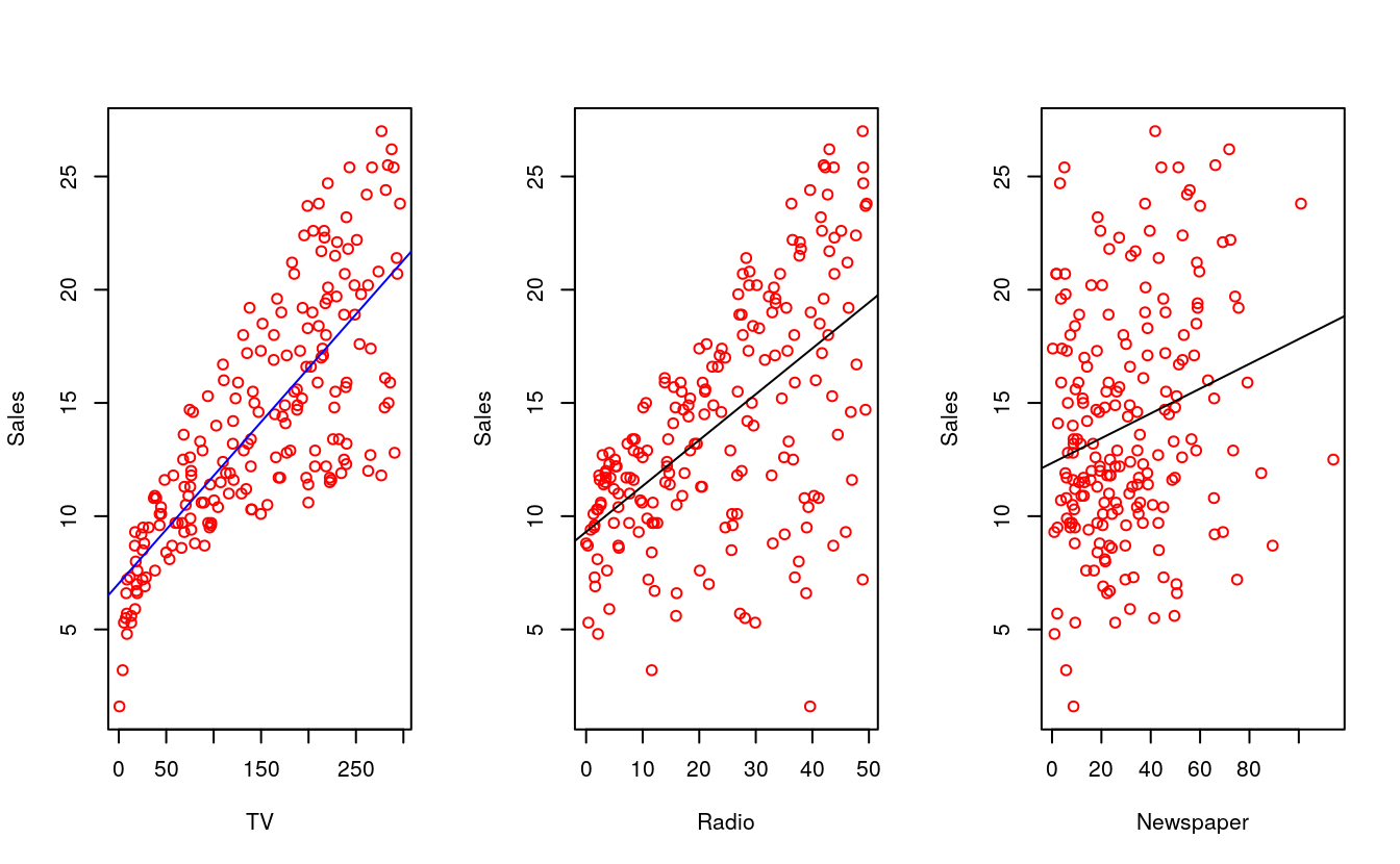
Recall the Advertising data from Chapter 2. Figure 2.1 displays sales (in thousands of units) for a particular product as a function of advertis- ing budgets (in thousands of dollars) for TV, radio, and newspaper media. Suppose that in our role as statistical consultants we are asked to suggest, on the basis of this data, a marketing plan for next year that will result in high product sales. What information would be useful in order to provide such a recommendation? Here are a few important questions that we might seek to address:
Is there a relationship between advertising budget and sales?
How strong is the relationship between advertising budget and sales?
Which media contribute to sales?
How accurately can we estimate the effect of each medium on sales?
For the Advertising data, the least squares fit for the regression of sales onto TV is shown. The fit is found by minimizing the sum of squared errors. Each grey line segment represents an error, and the fit makes a compro- mise by averaging their squares. In this case a linear fit captures the essence of the relationship, although it is somewhat deficient in the left of the plot.
tv_model <- lm(sales ~ TV, data = advertising)
plot(advertising$TV, advertising$sales, xlab = "TV", ylab = "Sales",
     col = "red", pch=16)
abline(tv_model, col = "blue", lwd=2)
segments(advertising$TV, advertising$sales, advertising$TV, predict(tv_model),
         col = "gray")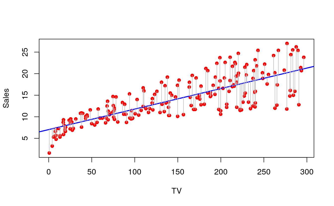
smry <- summary(tv_model)
smry
#>
#> Call:
#> lm(formula = sales ~ TV, data = advertising)
#>
#> Residuals:
#>    Min     1Q Median     3Q    Max
#> -8.386 -1.955 -0.191  2.067  7.212
#>
#> Coefficients:
#>             Estimate Std. Error t value Pr(>|t|)
#> (Intercept)  7.03259    0.45784    15.4   <2e-16 ***
#> TV           0.04754    0.00269    17.7   <2e-16 ***
#> ---
#> Signif. codes:  0 '***' 0.001 '**' 0.01 '*' 0.05 '.' 0.1 ' ' 1
#>
#> Residual standard error: 3.26 on 198 degrees of freedom
#> Multiple R-squared:  0.612,  Adjusted R-squared:  0.61
#> F-statistic:  312 on 1 and 198 DF,  p-value: <2e-16
library(lattice)

minRss <- sqrt(abs(min(smry$residuals))) * sign(min(smry$residuals))
maxRss <- sqrt(max(smry$residuals))

twovar <- function(x, y) {
  x^2 + y^2 }

mat <- outer( seq(minRss, maxRss, length = 100),
                seq(minRss, maxRss, length = 100),
                Vectorize( function(x,y) twovar(x, y) ) )


contourplot(mat, at = c(1,2,3))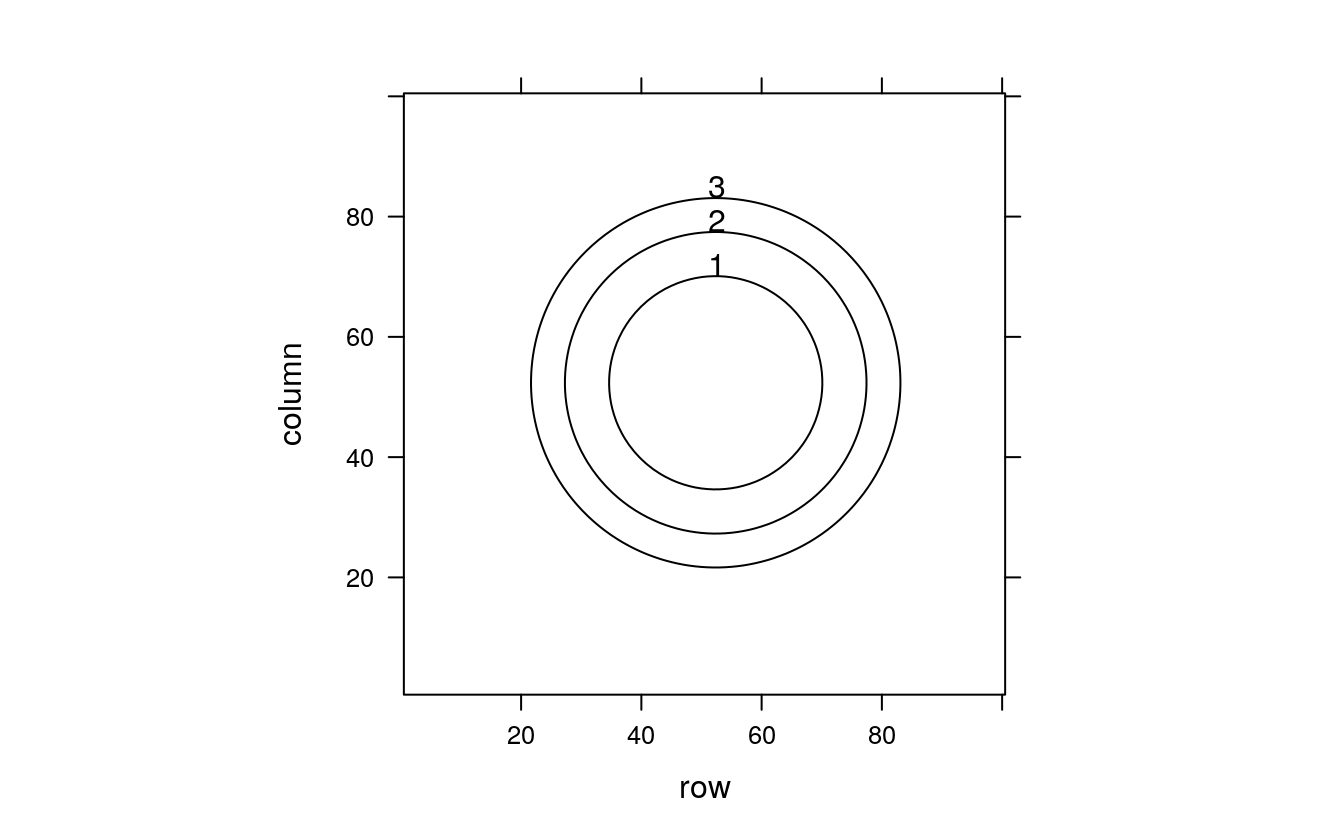
tv_model
#>
#> Call:
#> lm(formula = sales ~ TV, data = advertising)
#>
#> Coefficients:
#> (Intercept)           TV
#>      7.0326       0.0475
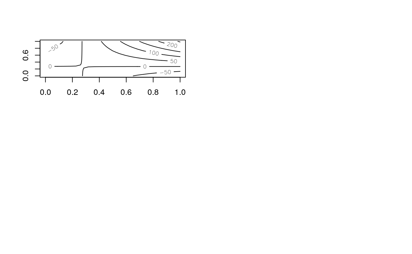
library(rsm)
mpg.lm <- lm(mpg ~ poly(hp, disp, degree = 3), data = mtcars)
contour(mpg.lm, hp ~ disp)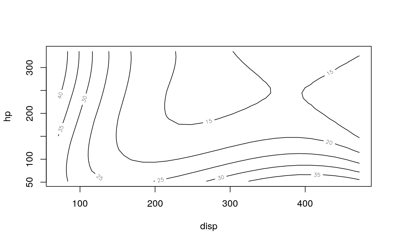
x <- -6:16
op <- par(mfrow = c(2, 2))
contour(outer(x, x), method = "flattest", vfont = c("sans serif", "plain"))