12 Feature Selection to enhance cancer detection
- Datasets:
breast-cancer-wisconsin.data - Algorithms:
- PCA
- Random Forest
- Recursive Feature Elimination
- Genetic Algorithm
Source: https://shiring.github.io/machine_learning/2017/01/15/rfe_ga_post
12.1 Read and process the data
bc_data <- read.table(file.path(data_raw_dir, "breast-cancer-wisconsin.data"),
                      header = FALSE, sep = ",")
# assign the column names
colnames(bc_data) <- c("sample_code_number", "clump_thickness",
                       "uniformity_of_cell_size", "uniformity_of_cell_shape",
                       "marginal_adhesion", "single_epithelial_cell_size",
                       "bare_nuclei", "bland_chromatin", "normal_nucleoli",
                       "mitosis", "classes")

# change classes from numeric to character
bc_data$classes <- ifelse(bc_data$classes == "2", "benign",
                          ifelse(bc_data$classes == "4", "malignant", NA))

# if query sign make NA
bc_data[bc_data == "?"] <- NA

# how many NAs are in the data
length(which(is.na(bc_data)))
#> [1] 16
names(bc_data)
#>  [1] "sample_code_number"          "clump_thickness"
#>  [3] "uniformity_of_cell_size"     "uniformity_of_cell_shape"
#>  [5] "marginal_adhesion"           "single_epithelial_cell_size"
#>  [7] "bare_nuclei"                 "bland_chromatin"
#>  [9] "normal_nucleoli"             "mitosis"
#> [11] "classes"
12.1.1 Missing data
# impute missing data
library(mice)
#>
#> Attaching package: 'mice'
#> The following objects are masked from 'package:base':
#>
#>     cbind, rbind

# skip these columns: sample_code_number and classes
# convert to numeric
bc_data[,2:10] <- apply(bc_data[, 2:10], 2, function(x) as.numeric(as.character(x)))

# impute but mute
dataset_impute <- mice(bc_data[, 2:10],  print = FALSE)

# bind "classes" with the rest. skip "sample_code_number"
bc_data <- cbind(bc_data[, 11, drop = FALSE],
                 mice::complete(dataset_impute, action =1))

bc_data$classes <- as.factor(bc_data$classes)

# how many benign and malignant cases are there?
summary(bc_data$classes)
#>    benign malignant
#>       458       241
str(bc_data)
#> 'data.frame':    699 obs. of  10 variables:
#>  $ classes                    : Factor w/ 2 levels "benign","malignant": 1 1 1 1 1 2 1 1 1 1 ...
#>  $ clump_thickness            : num  5 5 3 6 4 8 1 2 2 4 ...
#>  $ uniformity_of_cell_size    : num  1 4 1 8 1 10 1 1 1 2 ...
#>  $ uniformity_of_cell_shape   : num  1 4 1 8 1 10 1 2 1 1 ...
#>  $ marginal_adhesion          : num  1 5 1 1 3 8 1 1 1 1 ...
#>  $ single_epithelial_cell_size: num  2 7 2 3 2 7 2 2 2 2 ...
#>  $ bare_nuclei                : num  1 10 2 4 1 10 10 1 1 1 ...
#>  $ bland_chromatin            : num  3 3 3 3 3 9 3 3 1 2 ...
#>  $ normal_nucleoli            : num  1 2 1 7 1 7 1 1 1 1 ...
#>  $ mitosis                    : num  1 1 1 1 1 1 1 1 5 1 ...
12.2 Principal Component Analysis (PCA)
To get an idea about the dimensionality and variance of the datasets, I am first looking at PCA plots for samples and features. The first two principal components (PCs) show the two components that explain the majority of variation in the data.
After defining my custom ggplot2 theme, I am creating a function that performs the PCA (using the pcaGoPromoter package), calculates ellipses of the data points (with the ellipse package) and produces the plot with ggplot2. Some of the features in datasets 2 and 3 are not very distinct and overlap in the PCA plots, therefore I am also plotting hierarchical clustering dendrograms.
12.2.0.1 theme
# plotting theme

library(ggplot2)

my_theme <- function(base_size = 12, base_family = "sans"){
  theme_minimal(base_size = base_size, base_family = base_family) +
  theme(
    axis.text = element_text(size = 12),
    axis.text.x = element_text(angle = 0, vjust = 0.5, hjust = 0.5),
    axis.title = element_text(size = 14),
    panel.grid.major = element_line(color = "grey"),
    panel.grid.minor = element_blank(),
    panel.background = element_rect(fill = "aliceblue"),
    strip.background = element_rect(fill = "navy", color = "navy", size = 1),
    strip.text = element_text(face = "bold", size = 12, color = "white"),
    legend.position = "right",
    legend.justification = "top",
    legend.background = element_blank(),
    panel.border = element_rect(color = "grey", fill = NA, size = 0.5)
  )
}

theme_set(my_theme())
12.2.0.2 PCA function
# function for PCA plotting
library(pcaGoPromoter)                  # install from BioConductor
#> Loading required package: ellipse
#>
#> Attaching package: 'ellipse'
#> The following object is masked from 'package:graphics':
#>
#>     pairs
#> Loading required package: Biostrings
#> Loading required package: BiocGenerics
#> Loading required package: parallel
#>
#> Attaching package: 'BiocGenerics'
#> The following objects are masked from 'package:parallel':
#>
#>     clusterApply, clusterApplyLB, clusterCall, clusterEvalQ,
#>     clusterExport, clusterMap, parApply, parCapply, parLapply,
#>     parLapplyLB, parRapply, parSapply, parSapplyLB
#> The following objects are masked from 'package:mice':
#>
#>     cbind, rbind
#> The following objects are masked from 'package:stats':
#>
#>     IQR, mad, sd, var, xtabs
#> The following objects are masked from 'package:base':
#>
#>     anyDuplicated, append, as.data.frame, basename, cbind, colnames,
#>     dirname, do.call, duplicated, eval, evalq, Filter, Find, get, grep,
#>     grepl, intersect, is.unsorted, lapply, Map, mapply, match, mget,
#>     order, paste, pmax, pmax.int, pmin, pmin.int, Position, rank,
#>     rbind, Reduce, rownames, sapply, setdiff, sort, table, tapply,
#>     union, unique, unsplit, which, which.max, which.min
#> Loading required package: S4Vectors
#> Loading required package: stats4
#>
#> Attaching package: 'S4Vectors'
#> The following object is masked from 'package:base':
#>
#>     expand.grid
#> Loading required package: IRanges
#> Loading required package: XVector
#>
#> Attaching package: 'Biostrings'
#> The following object is masked from 'package:base':
#>
#>     strsplit
library(ellipse)

pca_func <- function(data, groups, title, print_ellipse = TRUE) {

  # perform pca and extract scores for all principal components: PC1:PC9
  pcaOutput <- pca(data, printDropped = FALSE, scale = TRUE, center = TRUE)
  pcaOutput2 <- as.data.frame(pcaOutput$scores)

  # define groups for plotting. will group the classes
  pcaOutput2$groups <- groups

  # when plotting samples calculate ellipses for plotting
  # (when plotting features, there are no replicates)
  if (print_ellipse) {
    # group and summarize by classes: benign, malignant
    # centroids w/3 columns: groups, PC1, PC2
    centroids <- aggregate(cbind(PC1, PC2) ~ groups, pcaOutput2, mean)
    # bind for the two groups (classes)
    # conf.rgn w/3 columns: groups, PC1, PC2
    conf.rgn  <- do.call(rbind, lapply(unique(pcaOutput2$groups), function(t)
      data.frame(groups = as.character(t),
                 # ellipse data for PC1 and PC2
                 ellipse(cov(pcaOutput2[pcaOutput2$groups == t, 1:2]),
                       centre = as.matrix(centroids[centroids$groups == t, 2:3]),
                       level = 0.95),
                 stringsAsFactors = FALSE)))

    plot <- ggplot(data = pcaOutput2, aes(x = PC1, y = PC2,
                                          group = groups,
                                          color = groups)) +
      geom_polygon(data = conf.rgn, aes(fill = groups), alpha = 0.2) + # ellipses
      geom_point(size = 2, alpha = 0.6) +
      scale_color_brewer(palette = "Set1") +
      labs(title = title,
           color = "",
           fill = "",
           x = paste0("PC1: ", round(pcaOutput$pov[1], digits = 2) * 100,
                      "% variance"),
           y = paste0("PC2: ", round(pcaOutput$pov[2], digits = 2) * 100,
                      "% variance"))

  } else {

    # if < 10 groups (e.g. the predictor classes) have colors from RColorBrewer
    if (length(unique(pcaOutput2$groups)) <= 10) {

      plot <- ggplot(data = pcaOutput2, aes(x = PC1, y = PC2,
                                            group = groups,
                                            color = groups)) +
        geom_point(size = 2, alpha = 0.6) +
        scale_color_brewer(palette = "Set1") +
        labs(title = title,
             color = "",
             fill = "",
             x = paste0("PC1: ", round(pcaOutput$pov[1], digits = 2) * 100,
                        "% variance"),
             y = paste0("PC2: ", round(pcaOutput$pov[2], digits = 2) * 100,
                        "% variance"))

    } else {
      # otherwise use the default rainbow colors
      plot <- ggplot(data = pcaOutput2, aes(x = PC1, y = PC2,
                                            group = groups, color = groups)) +
        geom_point(size = 2, alpha = 0.6) +
        labs(title = title,
             color = "",
             fill = "",
             x = paste0("PC1: ", round(pcaOutput$pov[1], digits = 2) * 100,
                        "% variance"),
             y = paste0("PC2: ", round(pcaOutput$pov[2], digits = 2) * 100,
                        "% variance"))
    }
  }

  return(plot)

}
library(gridExtra)
#>
#> Attaching package: 'gridExtra'
#> The following object is masked from 'package:BiocGenerics':
#>
#>     combine
library(grid)

# plot all data. one row is a feature
p1 <- pca_func(data = t(bc_data[, 2:10]),
               groups = as.character(bc_data$classes),
               title = "Breast cancer dataset 1: Samples")

# plot features only. features as columns
p2 <- pca_func(data = bc_data[, 2:10],
               groups = as.character(colnames(bc_data[, 2:10])),
               title = "Breast cancer dataset 1: Features", print_ellipse = FALSE)

grid.arrange(p1, p2, ncol = 2)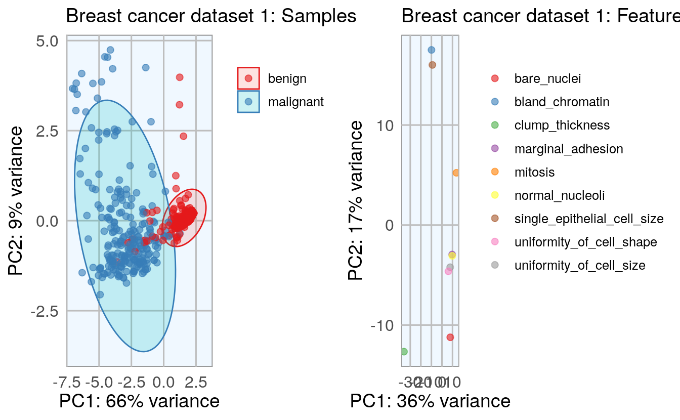

12.2.1 density plots vs class
# density plot showing the feature vs classes
library(tidyr)
#>
#> Attaching package: 'tidyr'
#> The following object is masked from 'package:S4Vectors':
#>
#>     expand

# gather data. from column clump_thickness to mitosis
bc_data_gather <- bc_data %>%
  gather(measure, value, clump_thickness:mitosis)

ggplot(data = bc_data_gather, aes(x = value, fill = classes, color = classes)) +
  geom_density(alpha = 0.3, size = 1) +
  geom_rug() +
  scale_fill_brewer(palette = "Set1") +
  scale_color_brewer(palette = "Set1") +
  facet_wrap( ~ measure, scales = "free_y", ncol = 3)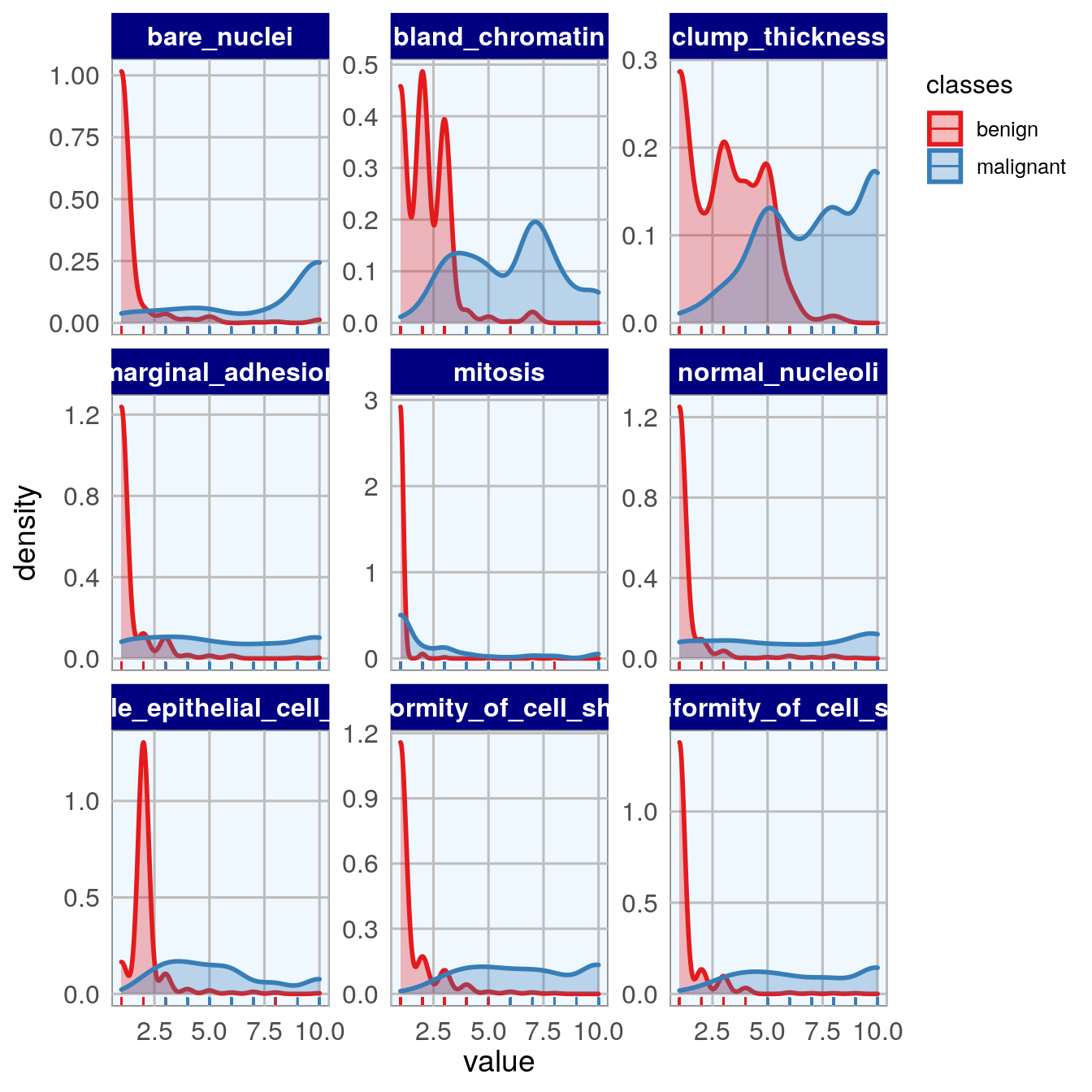
12.3 Feature importance
To get an idea about the feature’s respective importances, I’m running Random Forest models with 10 x 10 cross validation using the caret package. If I wanted to use feature importance to select features for modeling, I would need to perform it on the training data instead of on the complete dataset. But here, I only want to use it to get acquainted with my data. I am again defining a function that estimates the feature importance and produces a plot.
library(caret)
#> Loading required package: lattice
# library(doParallel) # parallel processing
# registerDoParallel()

# prepare training scheme
control <- trainControl(method = "repeatedcv", number = 10, repeats = 10)
feature_imp <- function(model, title) {
  # estimate variable importance
  importance <- varImp(model, scale = TRUE)
  # prepare dataframes for plotting
  importance_df_1 <- importance$importance
  importance_df_1$group <- rownames(importance_df_1)

  importance_df_2 <- importance_df_1
  importance_df_2$Overall <- 0
  importance_df <- rbind(importance_df_1, importance_df_2)

  plot <- ggplot() +
    geom_point(data = importance_df_1, aes(x = Overall,
                                           y = group,
                                           color = group), size = 2) +
    geom_path(data = importance_df, aes(x = Overall,
                                        y = group,
                                        color = group,
                                        group = group), size = 1) +
    theme(legend.position = "none") +
    labs(
      x = "Importance",
      y = "",
      title = title,
      subtitle = "Scaled feature importance",
      caption = "\nDetermined with Random Forest and
      repeated cross validation (10 repeats, 10 times)"
    )
  return(plot)
}
# train the model
set.seed(27)
imp_1 <- train(classes ~ ., data = bc_data, method = "rf",
               preProcess = c("scale", "center"),
               trControl = control)
p1 <- feature_imp(imp_1, title = "Breast cancer dataset 1")
p1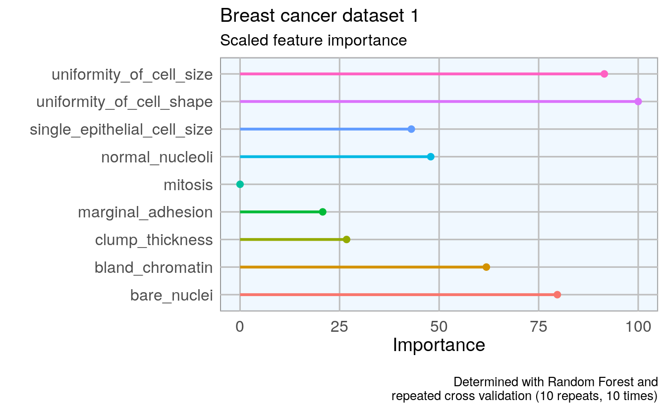
12.4 Feature Selection
- By correlation
- By Recursive Feature Elimination
- By Genetic Algorithm
set.seed(27)
bc_data_index <- createDataPartition(bc_data$classes, p = 0.7, list = FALSE)
bc_data_train <- bc_data[bc_data_index, ]
bc_data_test  <- bc_data[-bc_data_index, ]
12.4.1 Correlation
library(corrplot)
#> corrplot 0.84 loaded

# calculate correlation matrix
corMatMy <- cor(bc_data_train[, -1])
corrplot(corMatMy, order = "hclust")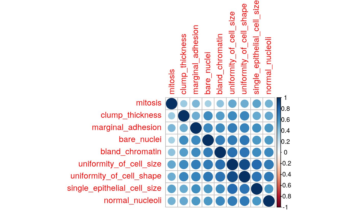
# Apply correlation filter at 0.70,
highlyCor <- colnames(bc_data_train[, -1])[findCorrelation(corMatMy,
                                                           cutoff = 0.7,
                                                           verbose = TRUE)]
#> Compare row 2  and column  3 with corr  0.9
#>   Means:  0.709 vs 0.595 so flagging column 2
#> Compare row 3  and column  7 with corr  0.737
#>   Means:  0.674 vs 0.572 so flagging column 3
#> All correlations <= 0.7
# which variables are flagged for removal?
highlyCor
#> [1] "uniformity_of_cell_size"  "uniformity_of_cell_shape"
# then we remove these variables
bc_data_cor <- bc_data_train[, which(!colnames(bc_data_train) %in% highlyCor)]
names(bc_data_cor)
#> [1] "classes"                     "clump_thickness"
#> [3] "marginal_adhesion"           "single_epithelial_cell_size"
#> [5] "bare_nuclei"                 "bland_chromatin"
#> [7] "normal_nucleoli"             "mitosis"
# confirm features were removed
outersect <- function(x, y) {
  sort(c(setdiff(x, y),
         setdiff(y, x)))
}

outersect(names(bc_data_cor), names(bc_data_train))
#> [1] "uniformity_of_cell_shape" "uniformity_of_cell_size"
Four features removed
12.4.2 Recursive Feature Elimination (RFE)
# ensure the results are repeatable
set.seed(7)

# define the control using a random forest selection function with cross validation
control <- rfeControl(functions = rfFuncs, method = "cv", number = 10)

# run the RFE algorithm
results_1 <- rfe(x = bc_data_train[, -1],
                 y = bc_data_train$classes,
                 sizes = c(1:9),
                 rfeControl = control)

# chosen features
predictors(results_1)
#> [1] "bare_nuclei"                 "clump_thickness"
#> [3] "normal_nucleoli"             "uniformity_of_cell_size"
#> [5] "uniformity_of_cell_shape"    "single_epithelial_cell_size"
#> [7] "bland_chromatin"             "marginal_adhesion"
# subset the chosen features
sel_cols <- which(colnames(bc_data_train) %in% predictors(results_1))
bc_data_rfe <- bc_data_train[, c(1, sel_cols)]
names(bc_data_rfe)
#> [1] "classes"                     "clump_thickness"
#> [3] "uniformity_of_cell_size"     "uniformity_of_cell_shape"
#> [5] "marginal_adhesion"           "single_epithelial_cell_size"
#> [7] "bare_nuclei"                 "bland_chromatin"
#> [9] "normal_nucleoli"
# confirm features removed by RFE
outersect(names(bc_data_rfe), names(bc_data_train))
#> [1] "mitosis"
No features removed with RFE
12.4.3 Genetic Algorithm (GA)
library(dplyr)
#>
#> Attaching package: 'dplyr'
#> The following object is masked from 'package:gridExtra':
#>
#>     combine
#> The following objects are masked from 'package:Biostrings':
#>
#>     collapse, intersect, setdiff, setequal, union
#> The following object is masked from 'package:XVector':
#>
#>     slice
#> The following objects are masked from 'package:IRanges':
#>
#>     collapse, desc, intersect, setdiff, slice, union
#> The following objects are masked from 'package:S4Vectors':
#>
#>     first, intersect, rename, setdiff, setequal, union
#> The following objects are masked from 'package:BiocGenerics':
#>
#>     combine, intersect, setdiff, union
#> The following objects are masked from 'package:stats':
#>
#>     filter, lag
#> The following objects are masked from 'package:base':
#>
#>     intersect, setdiff, setequal, union

ga_ctrl <- gafsControl(functions = rfGA, # Assess fitness with RF
                       method = "cv",    # 10 fold cross validation
                       genParallel = TRUE, # Use parallel programming
                       allowParallel = TRUE)

lev <- c("malignant", "benign")     # Set the levels

set.seed(27)
model_1 <- gafs(x = bc_data_train[, -1], y = bc_data_train$classes,
                   iters = 10, # generations of algorithm
                   popSize = 5, # population size for each generation
                   levels = lev,
                   gafsControl = ga_ctrl)
#>
#> Attaching package: 'recipes'
#> The following object is masked from 'package:stats':
#>
#>     step
plot(model_1) # Plot mean fitness (AUC) by generation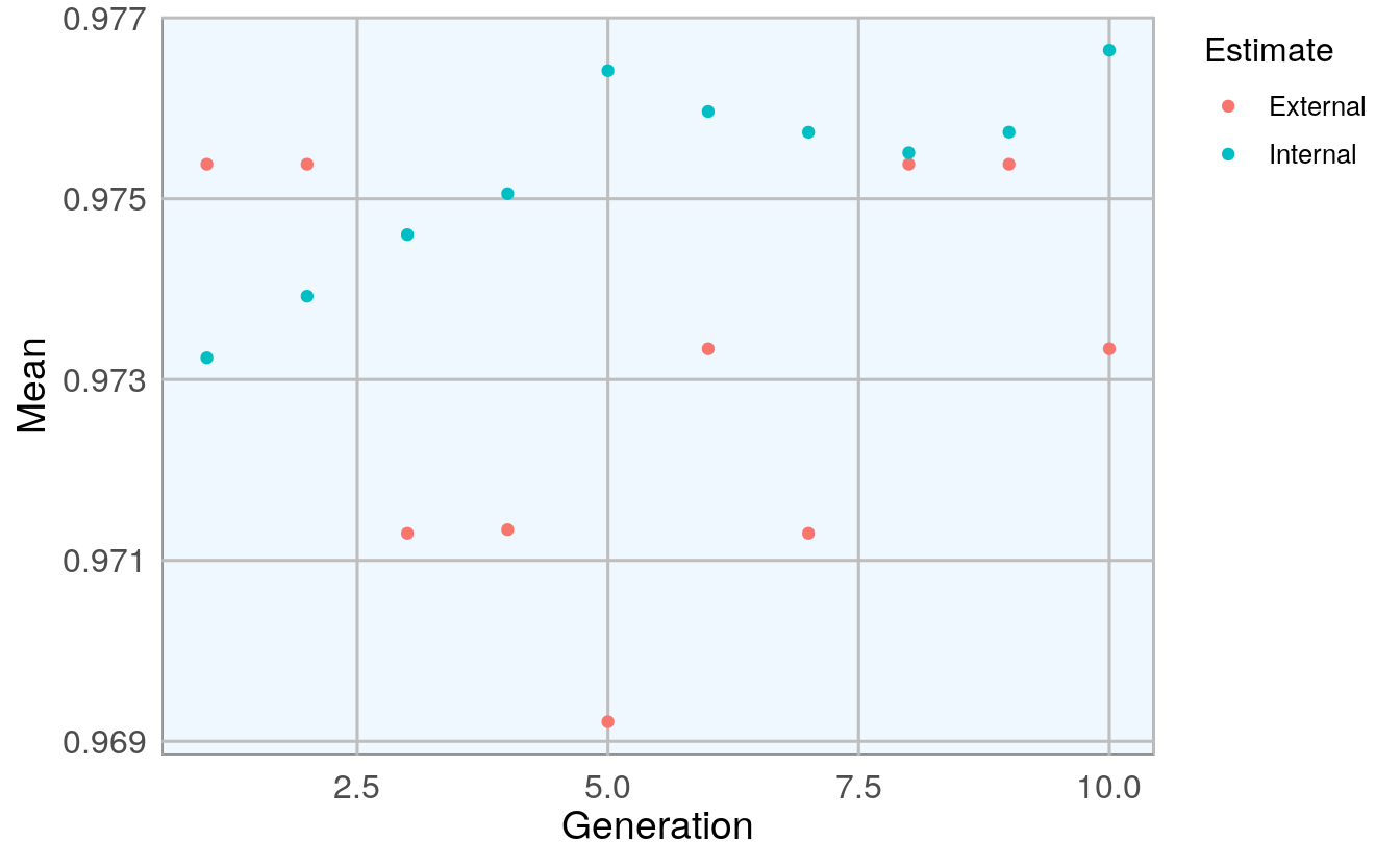
# features
model_1$ga$final
#> [1] "clump_thickness"          "uniformity_of_cell_size"
#> [3] "uniformity_of_cell_shape" "marginal_adhesion"
#> [5] "bare_nuclei"              "bland_chromatin"
#> [7] "normal_nucleoli"
# select features
sel_cols_ga <- which(colnames(bc_data_train) %in% model_1$ga$final)
bc_data_ga <- bc_data_train[, c(1, sel_cols_ga)]
names(bc_data_ga)
#> [1] "classes"                  "clump_thickness"
#> [3] "uniformity_of_cell_size"  "uniformity_of_cell_shape"
#> [5] "marginal_adhesion"        "bare_nuclei"
#> [7] "bland_chromatin"          "normal_nucleoli"
# features removed GA
outersect(names(bc_data_ga), names(bc_data_train))
#> [1] "mitosis"                     "single_epithelial_cell_size"
Two features removed with GA.
12.5 Model comparison
12.5.1 Using all features
set.seed(27)
model_bc_data_all <- train(classes ~ .,
                           data = bc_data_train,
                           method = "rf",
                           preProcess = c("scale", "center"),
                           trControl = trainControl(method = "repeatedcv",
                                                    number = 5, repeats = 10,
                                                    verboseIter = FALSE))
# confusion matrix
cm_all_1 <- confusionMatrix(predict(model_bc_data_all, bc_data_test[, -1]), bc_data_test$classes)
cm_all_1
#> Confusion Matrix and Statistics
#>
#>            Reference
#> Prediction  benign malignant
#>   benign       131         2
#>   malignant      6        70
#>
#>                Accuracy : 0.962
#>                  95% CI : (0.926, 0.983)
#>     No Information Rate : 0.656
#>     P-Value [Acc > NIR] : <2e-16
#>
#>                   Kappa : 0.916
#>
#>  Mcnemar's Test P-Value : 0.289
#>
#>             Sensitivity : 0.956
#>             Specificity : 0.972
#>          Pos Pred Value : 0.985
#>          Neg Pred Value : 0.921
#>              Prevalence : 0.656
#>          Detection Rate : 0.627
#>    Detection Prevalence : 0.636
#>       Balanced Accuracy : 0.964
#>
#>        'Positive' Class : benign
#>
12.5.2 Compare selection methods
# compare features selected by the three methods
library(gplots)
#>
#> Attaching package: 'gplots'
#> The following object is masked from 'package:IRanges':
#>
#>     space
#> The following object is masked from 'package:S4Vectors':
#>
#>     space
#> The following object is masked from 'package:stats':
#>
#>     lowess

venn_list <- list(cor = colnames(bc_data_cor)[-1],
                  rfe = colnames(bc_data_rfe)[-1],
                  ga  = colnames(bc_data_ga)[-1])

venn <- venn(venn_list)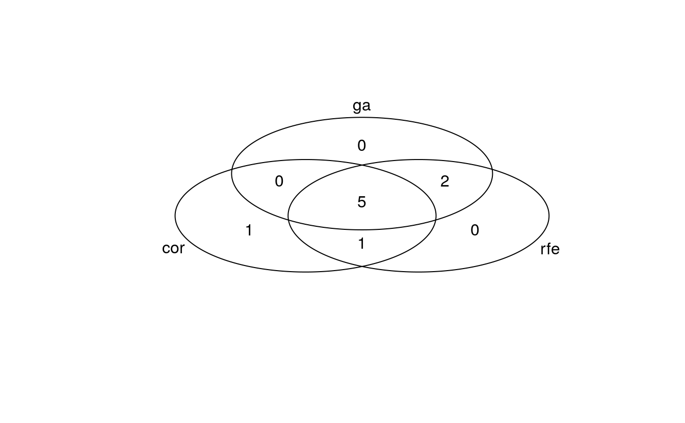
venn
#>     num cor rfe ga
#> 000   0   0   0  0
#> 001   0   0   0  1
#> 010   0   0   1  0
#> 011   2   0   1  1
#> 100   1   1   0  0
#> 101   0   1   0  1
#> 110   1   1   1  0
#> 111   5   1   1  1
#> attr(,"intersections")
#> attr(,"intersections")$`cor:rfe:ga`
#> [1] "clump_thickness"   "marginal_adhesion" "bare_nuclei"
#> [4] "bland_chromatin"   "normal_nucleoli"
#>
#> attr(,"intersections")$cor
#> [1] "mitosis"
#>
#> attr(,"intersections")$`rfe:ga`
#> [1] "uniformity_of_cell_size"  "uniformity_of_cell_shape"
#>
#> attr(,"intersections")$`cor:rfe`
#> [1] "single_epithelial_cell_size"
#>
#> attr(,"class")
#> [1] "venn"
4 out of 10 features were chosen by all three methods; the biggest overlap is seen between GA and RFE with 7 features. RFE and GA both retained 8 features for modeling, compared to only 5 based on the correlation method.
12.5.3 Correlation
# correlation
set.seed(127)
model_bc_data_cor <- train(classes ~ .,
                 data = bc_data_cor,
                 method = "rf",
                 preProcess = c("scale", "center"),
                 trControl = trainControl(method = "repeatedcv", number = 5, repeats = 10, verboseIter = FALSE))
cm_cor_1 <- confusionMatrix(predict(model_bc_data_cor, bc_data_test[, -1]), bc_data_test$classes)
cm_cor_1
#> Confusion Matrix and Statistics
#>
#>            Reference
#> Prediction  benign malignant
#>   benign       130         4
#>   malignant      7        68
#>
#>                Accuracy : 0.947
#>                  95% CI : (0.908, 0.973)
#>     No Information Rate : 0.656
#>     P-Value [Acc > NIR] : <2e-16
#>
#>                   Kappa : 0.885
#>
#>  Mcnemar's Test P-Value : 0.546
#>
#>             Sensitivity : 0.949
#>             Specificity : 0.944
#>          Pos Pred Value : 0.970
#>          Neg Pred Value : 0.907
#>              Prevalence : 0.656
#>          Detection Rate : 0.622
#>    Detection Prevalence : 0.641
#>       Balanced Accuracy : 0.947
#>
#>        'Positive' Class : benign
#>
12.5.4 Recursive Feature Elimination
set.seed(127)
model_bc_data_rfe <- train(classes ~ .,
                           data = bc_data_rfe,
                           method = "rf",
                           preProcess = c("scale", "center"),
                           trControl = trainControl(method = "repeatedcv",
                                                    number = 5, repeats = 10,
                                                    verboseIter = FALSE))
cm_rfe_1 <- confusionMatrix(predict(model_bc_data_rfe, bc_data_test[, -1]), bc_data_test$classes)
cm_rfe_1
#> Confusion Matrix and Statistics
#>
#>            Reference
#> Prediction  benign malignant
#>   benign       130         3
#>   malignant      7        69
#>
#>                Accuracy : 0.952
#>                  95% CI : (0.914, 0.977)
#>     No Information Rate : 0.656
#>     P-Value [Acc > NIR] : <2e-16
#>
#>                   Kappa : 0.895
#>
#>  Mcnemar's Test P-Value : 0.343
#>
#>             Sensitivity : 0.949
#>             Specificity : 0.958
#>          Pos Pred Value : 0.977
#>          Neg Pred Value : 0.908
#>              Prevalence : 0.656
#>          Detection Rate : 0.622
#>    Detection Prevalence : 0.636
#>       Balanced Accuracy : 0.954
#>
#>        'Positive' Class : benign
#>
12.5.5 GA
set.seed(127)
model_bc_data_ga <- train(classes ~ .,
                           data = bc_data_ga,
                           method = "rf",
                           preProcess = c("scale", "center"),
                           trControl = trainControl(method = "repeatedcv",
                                                    number = 5, repeats = 10,
                                                    verboseIter = FALSE))
cm_ga_1 <- confusionMatrix(predict(model_bc_data_ga, bc_data_test[, -1]), bc_data_test$classes)
cm_ga_1
#> Confusion Matrix and Statistics
#>
#>            Reference
#> Prediction  benign malignant
#>   benign       131         2
#>   malignant      6        70
#>
#>                Accuracy : 0.962
#>                  95% CI : (0.926, 0.983)
#>     No Information Rate : 0.656
#>     P-Value [Acc > NIR] : <2e-16
#>
#>                   Kappa : 0.916
#>
#>  Mcnemar's Test P-Value : 0.289
#>
#>             Sensitivity : 0.956
#>             Specificity : 0.972
#>          Pos Pred Value : 0.985
#>          Neg Pred Value : 0.921
#>              Prevalence : 0.656
#>          Detection Rate : 0.627
#>    Detection Prevalence : 0.636
#>       Balanced Accuracy : 0.964
#>
#>        'Positive' Class : benign
#>
12.6 Create comparison tables
# take "overall" variable only from Confusion Matrix
overall <- data.frame(dataset = 1,
           model = rep(c("all", "cor", "rfe", "ga"), 1),
           rbind(cm_all_1$overall,
                 cm_cor_1$overall,
                 cm_rfe_1$overall,
                 cm_ga_1$overall)
)

# convert to tidy data
library(tidyr)
overall_gather <- overall[, 1:4] %>%     # take the first columns:
  gather(measure, value, Accuracy:Kappa) # dataset, model, Accuracy and Kappa
# take "byClass" variable only from Confusion Matrix
byClass <- data.frame(dataset = 1,
                      model = rep(c("all", "cor", "rfe", "ga"), 1),
                      rbind(cm_all_1$byClass,
                      cm_cor_1$byClass,
                      cm_rfe_1$byClass,
                      cm_ga_1$byClass)
)

# convert to tidy data
byClass_gather <- byClass[, c(1:4, 7)] %>%      # select columns: dataset, model
  gather(measure, value, Sensitivity:Precision) # Sensitiv, Specific, Precis
# join the two tables
overall_byClass_gather <- rbind(overall_gather, byClass_gather)
overall_byClass_gather <- within(
  overall_byClass_gather, model <- factor(model,
                                          levels = c("all", "cor", "rfe", "ga")))
                                          # convert to factor

ggplot(overall_byClass_gather, aes(x = model, y = value, color = measure,
                                   shape = measure, group = measure)) +
  geom_point(size = 4, alpha = 0.8) +
  geom_path(alpha = 0.7) +
  scale_colour_brewer(palette = "Set1") +
  facet_grid(dataset ~ ., scales = "free_y") +
  labs(
    x = "Feature Selection method",
    y = "Value",
    color = "",
    shape = "",
    title = "Comparison of feature selection methods",
    subtitle = "in three breast cancer datasets",
    caption = "\nBreast Cancer Wisconsin (Diagnostic) Data Sets: 1, 2 & 3
    Street et al., 1993;
    all: no feature selection
    cor: features with correlation > 0.7 removed
    rfe: Recursive Feature Elimination
    ga: Genetic Algorithm"
  )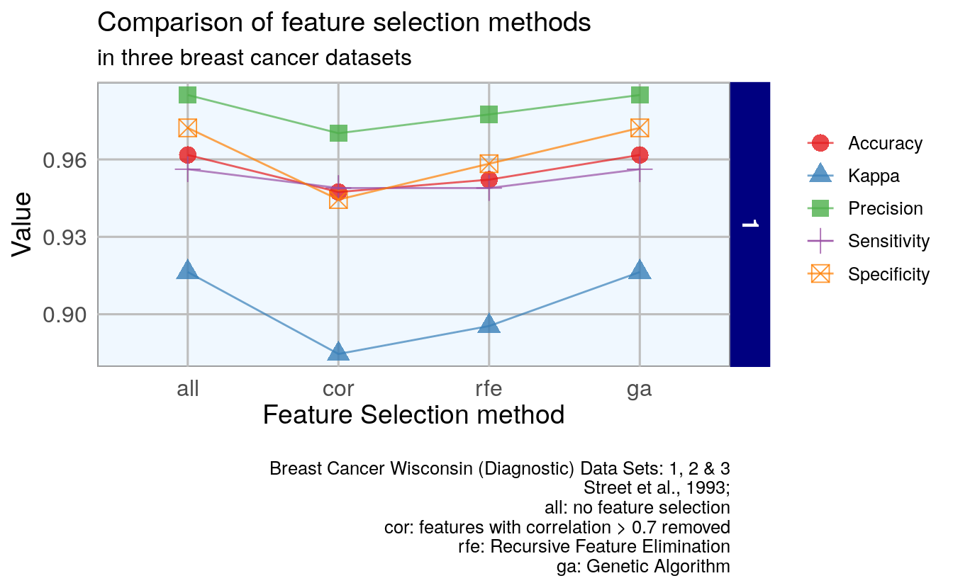
- Less accurate: selection of features by correlation
- More accurate: genetic algorithm
- Including all features is more accurate to removing features by correlation.