29 A detailed study of bike sharing demand

Datasets: bike-sharing-demand
Algorithms:
- Decision Trees
- Conditional Inference Tree
- Random Forest

#loading the required libraries
library(rpart)
library(rattle)
#> Rattle: A free graphical interface for data science with R.
#> Version 5.3.0 Copyright (c) 2006-2018 Togaware Pty Ltd.
#> Type 'rattle()' to shake, rattle, and roll your data.
library(rpart.plot)
library(RColorBrewer)
library(randomForest)
#> randomForest 4.6-14
#> Type rfNews() to see new features/changes/bug fixes.
#> 
#> Attaching package: 'randomForest'
#> The following object is masked from 'package:rattle':
#> 
#>     importance
library(corrplot)
#> corrplot 0.84 loaded
library(dplyr)
#> 
#> Attaching package: 'dplyr'
#> The following object is masked from 'package:randomForest':
#> 
#>     combine
#> The following objects are masked from 'package:stats':
#> 
#>     filter, lag
#> The following objects are masked from 'package:base':
#> 
#>     intersect, setdiff, setequal, union
library(tictoc)

Source: https://www.analyticsvidhya.com/blog/2015/06/solution-kaggle-competition-bike-sharing-demand/

29.1 Hypothesis Generation

Before exploring the data to understand the relationship between variables, I’d recommend you to focus on hypothesis generation first. Now, this might sound counter-intuitive for solving a data science problem, but if there is one thing I have learnt over years, it is this. Before exploring data, you should spend some time thinking about the business problem, gaining the domain knowledge and may be gaining first hand experience of the problem (only if I could travel to North America!)

How does it help? This practice usually helps you form better features later on, which are not biased by the data available in the dataset. At this stage, you are expected to posses structured thinking i.e. a thinking process which takes into consideration all the possible aspects of a particular problem.

Here are some of the hypothesis which I thought could influence the demand of bikes:

Hourly trend: There must be high demand during office timings. Early morning and late evening can have different trend (cyclist) and low demand during 10:00 pm to 4:00 am.
Daily Trend: Registered users demand more bike on weekdays as compared to weekend or holiday.
Rain: The demand of bikes will be lower on a rainy day as compared to a sunny day. Similarly, higher humidity will cause to lower the demand and vice versa.
Temperature: Would high or low temperature encourage or disencourage bike riding?
Pollution: If the pollution level in a city starts soaring, people may start using Bike (it may be influenced by government / company policies or increased awareness).
Time: Total demand should have higher contribution of registered user as compared to casual because registered user base would increase over time.
Traffic: It can be positively correlated with Bike demand. Higher traffic may force people to use bike as compared to other road transport medium like car, taxi etc

29.2 Understanding the Data Set

The dataset shows hourly rental data for two years (2011 and 2012). The training data set is for the first 19 days of each month. The test dataset is from 20th day to month’s end. We are required to predict the total count of bikes rented during each hour covered by the test set.

In the training data set, they have separately given bike demand by registered, casual users and sum of both is given as count.

Training data set has 12 variables (see below) and Test has 9 (excluding registered, casual and count).

29.2.1 Independent variables

datetime:   date and hour in "mm/dd/yyyy hh:mm" format
season:     Four categories-> 1 = spring, 2 = summer, 3 = fall, 4 = winter
holiday:    whether the day is a holiday or not (1/0)
workingday: whether the day is neither a weekend nor holiday (1/0)
weather:    Four Categories of weather
            1-> Clear, Few clouds, Partly cloudy, Partly cloudy
            2-> Mist + Cloudy, Mist + Broken clouds, Mist + Few clouds, Mist
            3-> Light Snow and Rain + Thunderstorm + Scattered clouds, Light Rain + Scattered clouds
            4-> Heavy Rain + Ice Pallets + Thunderstorm + Mist, Snow + Fog
temp:       hourly temperature in Celsius
atemp:      "feels like" temperature in Celsius
humidity:   relative humidity
windspeed:  wind speed

29.2.2 Dependent variables

registered: number of registered user
casual:     number of non-registered user
count:      number of total rentals (registered + casual)

29.3 Importing the dataset and Data Exploration

For this solution, I have used R (R Studio 0.99.442) in Windows Environment.

Below are the steps to import and perform data exploration. If you are new to this concept, you can refer this guide on Data Exploration in R

Import Train and Test Data Set

# https://www.kaggle.com/c/bike-sharing-demand/data
train = read.csv(file.path(data_raw_dir, "bike_train.csv"))
test = read.csv(file.path(data_raw_dir, "bike_test.csv"))

glimpse(train)
#> Rows: 10,886
#> Columns: 12
#> $ datetime   <fct> 2011-01-01 00:00:00, 2011-01-01 01:00:00, 2011-01-01 02:00…
#> $ season     <int> 1, 1, 1, 1, 1, 1, 1, 1, 1, 1, 1, 1, 1, 1, 1, 1, 1, 1, 1, 1…
#> $ holiday    <int> 0, 0, 0, 0, 0, 0, 0, 0, 0, 0, 0, 0, 0, 0, 0, 0, 0, 0, 0, 0…
#> $ workingday <int> 0, 0, 0, 0, 0, 0, 0, 0, 0, 0, 0, 0, 0, 0, 0, 0, 0, 0, 0, 0…
#> $ weather    <int> 1, 1, 1, 1, 1, 2, 1, 1, 1, 1, 1, 1, 1, 2, 2, 2, 2, 2, 3, 3…
#> $ temp       <dbl> 9.84, 9.02, 9.02, 9.84, 9.84, 9.84, 9.02, 8.20, 9.84, 13.1…
#> $ atemp      <dbl> 14.4, 13.6, 13.6, 14.4, 14.4, 12.9, 13.6, 12.9, 14.4, 17.4…
#> $ humidity   <int> 81, 80, 80, 75, 75, 75, 80, 86, 75, 76, 76, 81, 77, 72, 72…
#> $ windspeed  <dbl> 0, 0, 0, 0, 0, 6, 0, 0, 0, 0, 17, 19, 19, 20, 19, 20, 20, …
#> $ casual     <int> 3, 8, 5, 3, 0, 0, 2, 1, 1, 8, 12, 26, 29, 47, 35, 40, 41, …
#> $ registered <int> 13, 32, 27, 10, 1, 1, 0, 2, 7, 6, 24, 30, 55, 47, 71, 70, …
#> $ count      <int> 16, 40, 32, 13, 1, 1, 2, 3, 8, 14, 36, 56, 84, 94, 106, 11…
glimpse(test)
#> Rows: 6,493
#> Columns: 9
#> $ datetime   <fct> 2011-01-20 00:00:00, 2011-01-20 01:00:00, 2011-01-20 02:00…
#> $ season     <int> 1, 1, 1, 1, 1, 1, 1, 1, 1, 1, 1, 1, 1, 1, 1, 1, 1, 1, 1, 1…
#> $ holiday    <int> 0, 0, 0, 0, 0, 0, 0, 0, 0, 0, 0, 0, 0, 0, 0, 0, 0, 0, 0, 0…
#> $ workingday <int> 1, 1, 1, 1, 1, 1, 1, 1, 1, 1, 1, 1, 1, 1, 1, 1, 1, 1, 1, 1…
#> $ weather    <int> 1, 1, 1, 1, 1, 1, 1, 1, 1, 2, 1, 2, 2, 2, 2, 2, 2, 2, 2, 1…
#> $ temp       <dbl> 10.66, 10.66, 10.66, 10.66, 10.66, 9.84, 9.02, 9.02, 9.02,…
#> $ atemp      <dbl> 11.4, 13.6, 13.6, 12.9, 12.9, 11.4, 10.6, 10.6, 10.6, 11.4…
#> $ humidity   <int> 56, 56, 56, 56, 56, 60, 60, 55, 55, 52, 48, 45, 42, 45, 45…
#> $ windspeed  <dbl> 26, 0, 0, 11, 11, 15, 15, 15, 19, 15, 20, 11, 0, 7, 9, 13,…

Combine both Train and Test Data set (to understand the distribution of independent variable together).

# add variables to test dataset before merging
test$registered=0
test$casual=0
test$count=0

data = rbind(train,test)

Variable Type Identification

str(data)
#> 'data.frame':    17379 obs. of  12 variables:
#>  $ datetime  : Factor w/ 17379 levels "2011-01-01 00:00:00",..: 1 2 3 4 5 6 7 8 9 10 ...
#>  $ season    : int  1 1 1 1 1 1 1 1 1 1 ...
#>  $ holiday   : int  0 0 0 0 0 0 0 0 0 0 ...
#>  $ workingday: int  0 0 0 0 0 0 0 0 0 0 ...
#>  $ weather   : int  1 1 1 1 1 2 1 1 1 1 ...
#>  $ temp      : num  9.84 9.02 9.02 9.84 9.84 ...
#>  $ atemp     : num  14.4 13.6 13.6 14.4 14.4 ...
#>  $ humidity  : int  81 80 80 75 75 75 80 86 75 76 ...
#>  $ windspeed : num  0 0 0 0 0 ...
#>  $ casual    : num  3 8 5 3 0 0 2 1 1 8 ...
#>  $ registered: num  13 32 27 10 1 1 0 2 7 6 ...
#>  $ count     : num  16 40 32 13 1 1 2 3 8 14 ...

Find missing values in the dataset if any

table(is.na(data))
#> 
#>  FALSE 
#> 208548

No NAs in the dataset.

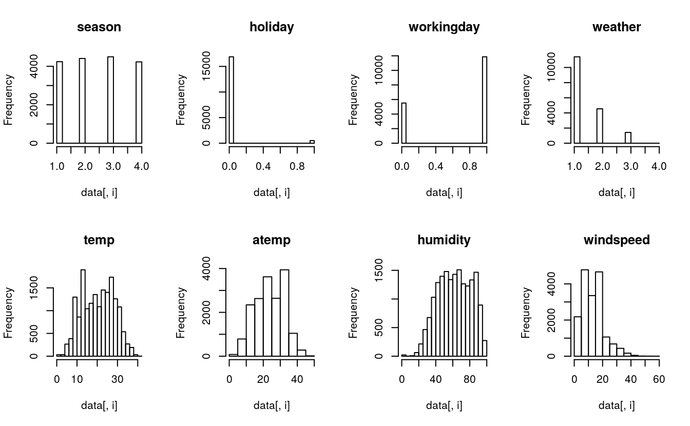
Understand the distribution of numerical variables and generate a frequency table for numeric variables. Analyze the distribution.

29.3.1 histograms

# histograms each attribute
par(mfrow=c(2,4))
for(i in 2:9) {
    hist(data[,i], main = names(data)[i])
}

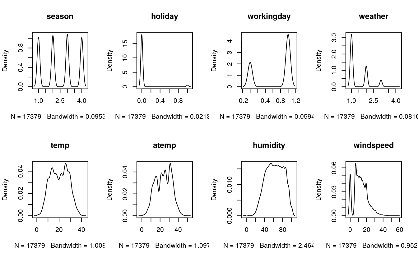
29.3.2 density plots

# density plot for each attribute
par(mfrow=c(2,4))
for(i in 2:9) {
    plot(density(data[,i]), main=names(data)[i])
}

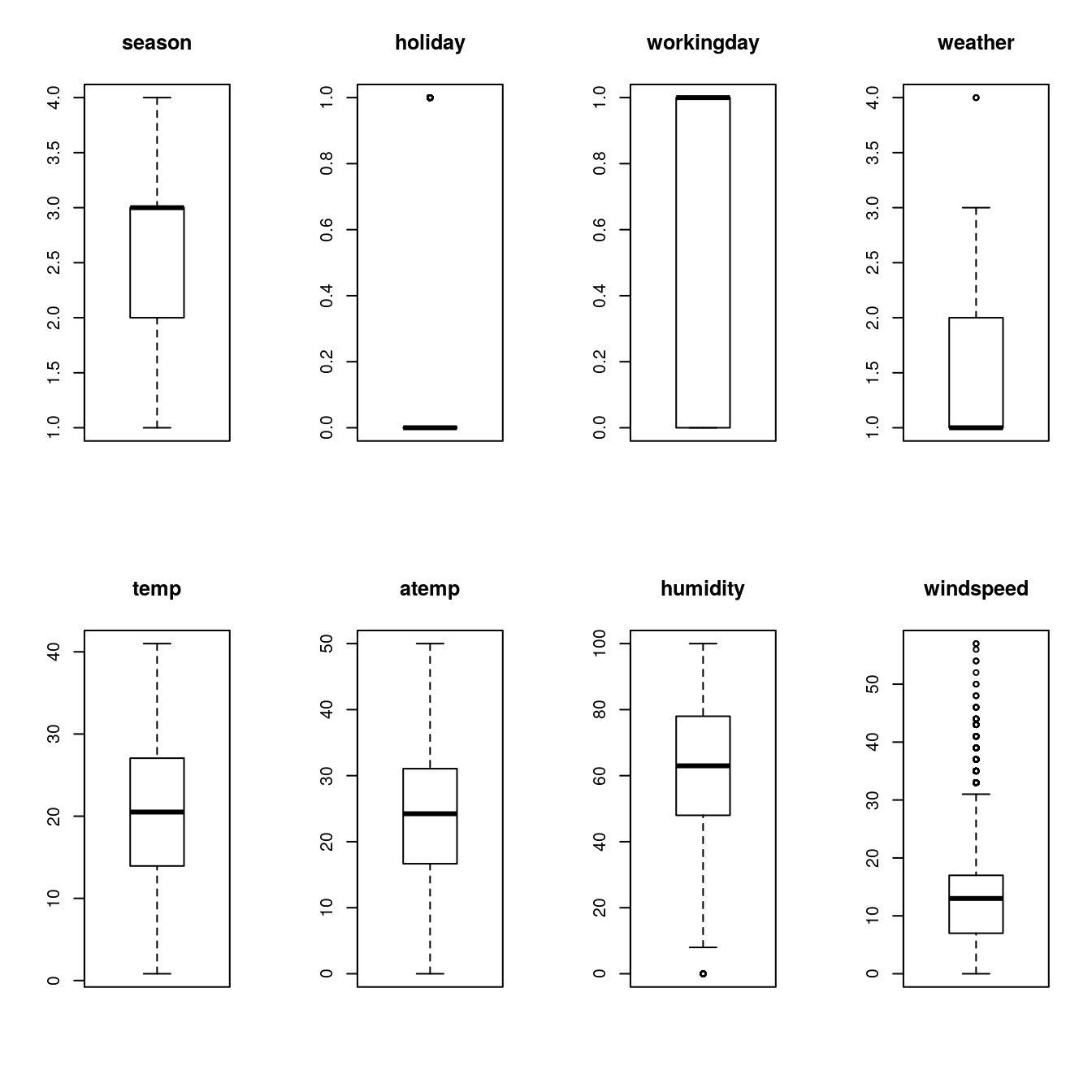
29.3.3 boxplots

# boxplots for each attribute
par(mfrow=c(2,4))
for(i in 2:9) {
    boxplot(data[,i], main=names(data)[i])
}

29.3.4 Unique values of discrete variables

# the discrete variables in this case are integers
ints <- unlist(lapply(data, is.integer))
names(data)[ints]
#> [1] "season"     "holiday"    "workingday" "weather"    "humidity"

Humidity should not be an integer or discrete variable; it is a continuous or numeric variable.

# convert humidity to numeric
data$humidity <- as.numeric(data$humidity)

# list unique values of integer variables
ints <- unlist(lapply(data, is.integer))
int_vars <- names(data)[ints]

sapply(int_vars, function(x) unique(data[x]))
#> $season.season
#> [1] 1 2 3 4
#> 
#> $holiday.holiday
#> [1] 0 1
#> 
#> $workingday.workingday
#> [1] 0 1
#> 
#> $weather.weather
#> [1] 1 2 3 4

29.3.5 Inferences

The variables season, holiday, workingday and weather are discrete (integer).
Activity is even through all seasons.
Most of the activitity happens during non-holidays.
Activity doubles during the working days.
Activity happens mostly during clear (1) weather.
temp, atemp and humidity are continuous variables (numeric).

29.4 Hypothesis Testing (using multivariate analysis)

Till now, we have got a fair understanding of the data set. Now, let’s test the hypothesis which we had generated earlier. Here I have added some additional hypothesis from the dataset. Let’s test them one by one:

29.4.1 Hourly trend

There must be high demand during office timings. Early morning and late evening can have different trend (cyclist) and low demand during 10:00 pm to 4:00 am.

We don’t have the variable ‘hour’ with us. But we can extract it using the datetime column.

head(data$datetime)
#> [1] 2011-01-01 00:00:00 2011-01-01 01:00:00 2011-01-01 02:00:00
#> [4] 2011-01-01 03:00:00 2011-01-01 04:00:00 2011-01-01 05:00:00
#> 17379 Levels: 2011-01-01 00:00:00 2011-01-01 01:00:00 ... 2012-12-31 23:00:00

class(data$datetime)
#> [1] "factor"

# show hour and day from the variable datetime
head(substr(data$datetime, 12, 13))  # hour
#> [1] "00" "01" "02" "03" "04" "05"
head(substr(data$datetime, 9, 10))   # day
#> [1] "01" "01" "01" "01" "01" "01"

# extracting hour
data$hour = substr(data$datetime,12,13)
data$hour = as.factor(data$hour)
head(data$hour)
#> [1] 00 01 02 03 04 05
#> 24 Levels: 00 01 02 03 04 05 06 07 08 09 10 11 12 13 14 15 16 17 18 19 ... 23

### dividing again in train and test
# the train dataset is for the first 19 days
train = data[as.integer(substr(data$datetime, 9, 10)) < 20,]

# the test dataset is from day 20 to the end of the month
test = data[as.integer(substr(data$datetime, 9, 10)) > 19,]

29.4.2 boxplot count vs hour in training set

boxplot(train$count ~ train$hour, xlab="hour", ylab="count of users")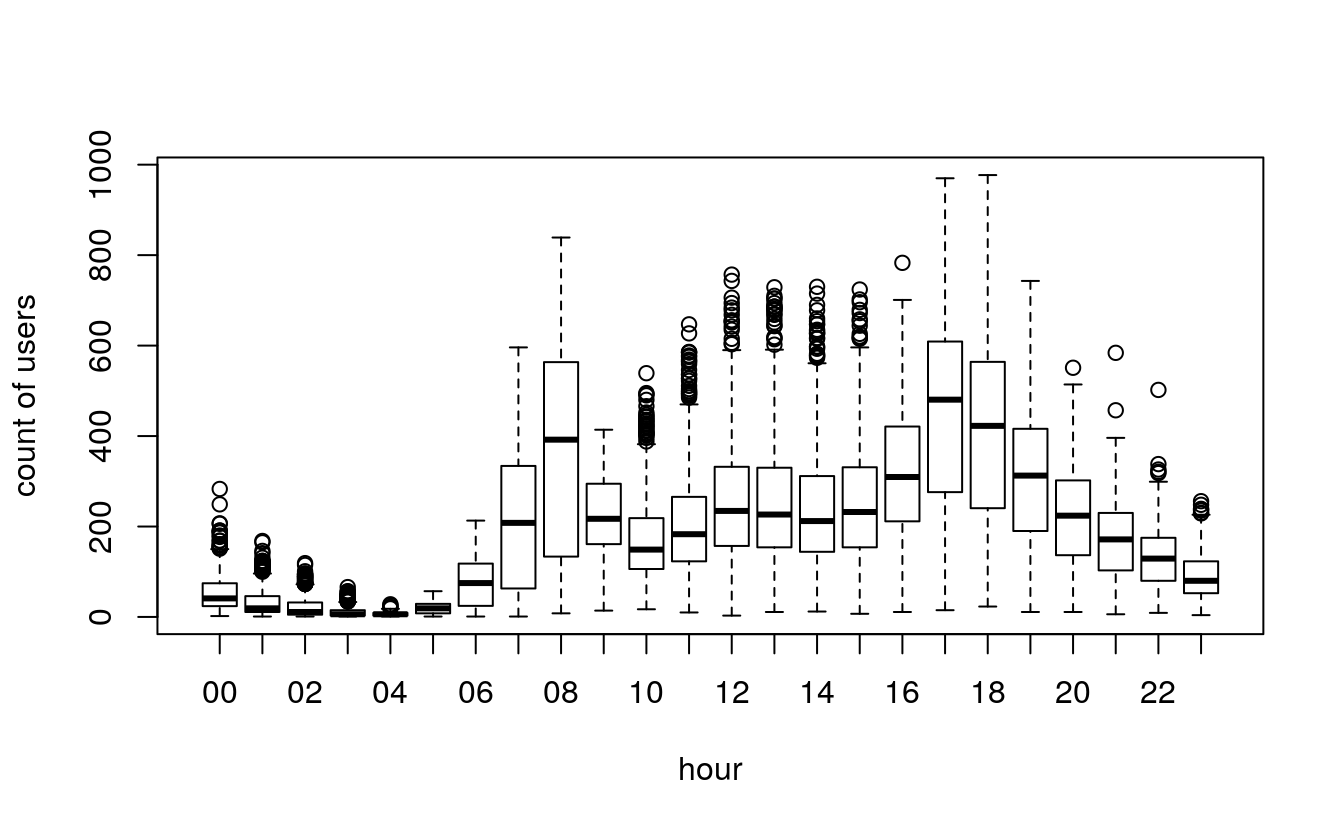

Rides increase from 6 am to 6pm, during office hours.

# casual users
casual <- data[data$casual > 0, ]
registered <- data[data$registered > 0, ]

dim(casual)
#> [1] 9900   13
dim(registered)
#> [1] 10871    13

29.4.3 Boxplot hourly: casual vs registered users in the training set

# by hour: casual vs registered users
par(mfrow=c(2,1))
boxplot(train$casual ~ train$hour, xlab="hour", ylab="casual users")
boxplot(train$registered ~ train$hour, xlab="hour", ylab="registered users")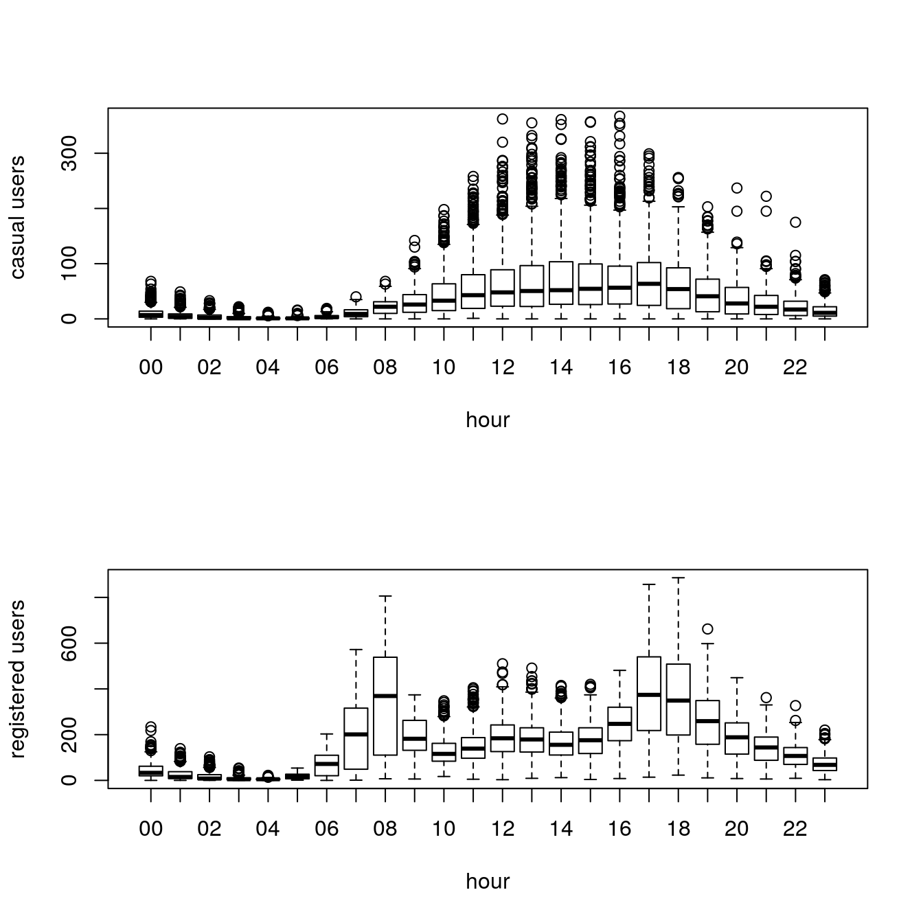

Casual and Registered users have different distributions. Casual users tend to rent more during office hours.

29.4.4 outliers in the training set

par(mfrow=c(2,1))
boxplot(train$count ~ train$hour, xlab="hour", ylab="count of users")
boxplot(log(train$count) ~ train$hour,xlab="hour",ylab="log(count)")

29.4.5 Daily trend

Registered users demand more bike on weekdays as compared to weekend or holiday.

# extracting days of week
date <- substr(data$datetime, 1, 10)
days <- weekdays(as.Date(date))
data$day <- days

# split the dataset again at day 20 of the month, before and after
train = data[as.integer(substr(data$datetime,9,10)) < 20,]
test  = data[as.integer(substr(data$datetime,9,10)) > 19,]

29.4.6 Boxplot daily trend: casual vs registered users, training set

# creating boxplots for rentals with different variables to see the variation
par(mfrow=c(2,1))
boxplot(train$casual ~ train$day, xlab="day", ylab="casual users")
boxplot(train$registered ~ train$day, xlab="day", ylab="registered users")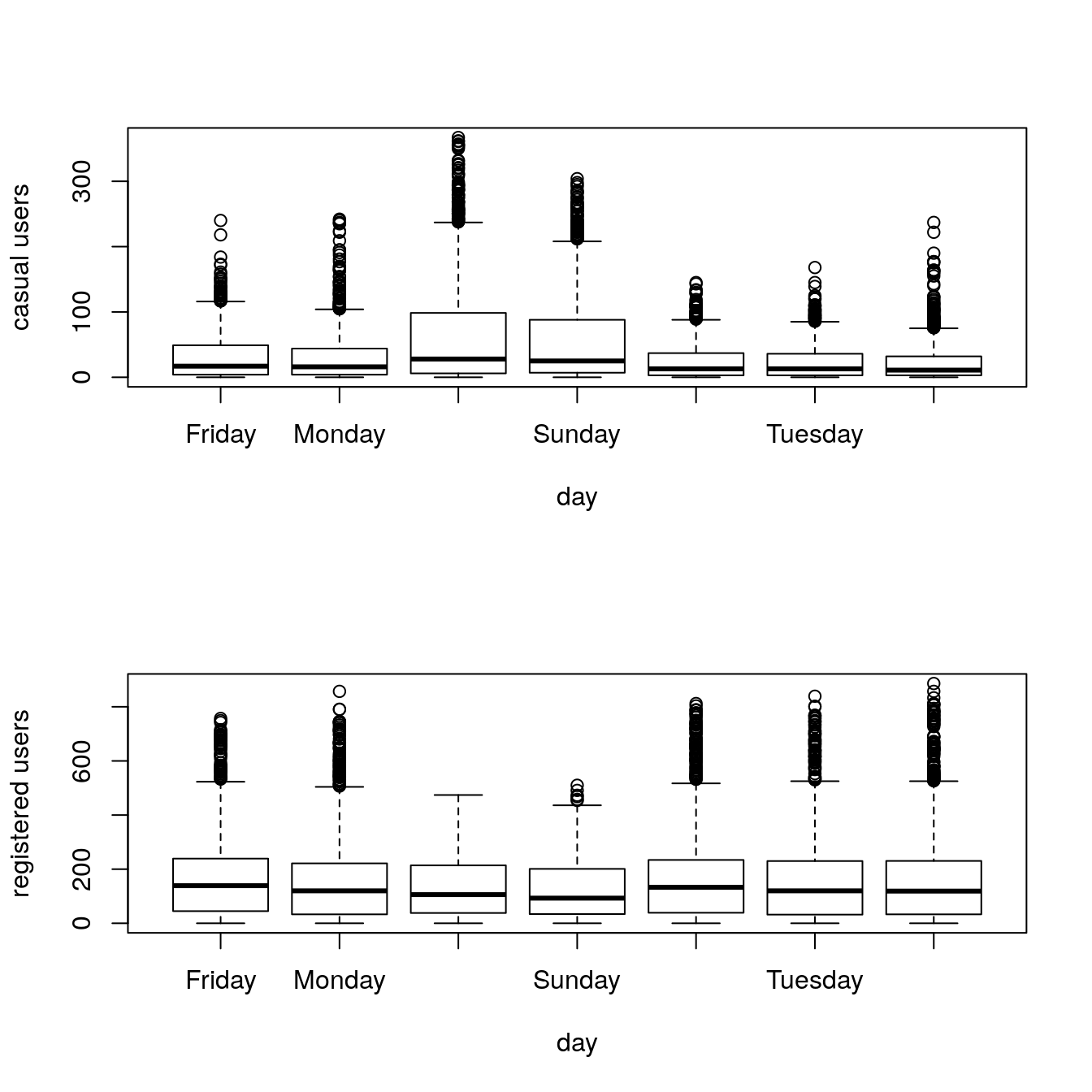

Demand of casual users increases during the weekend, contrary of registered users.

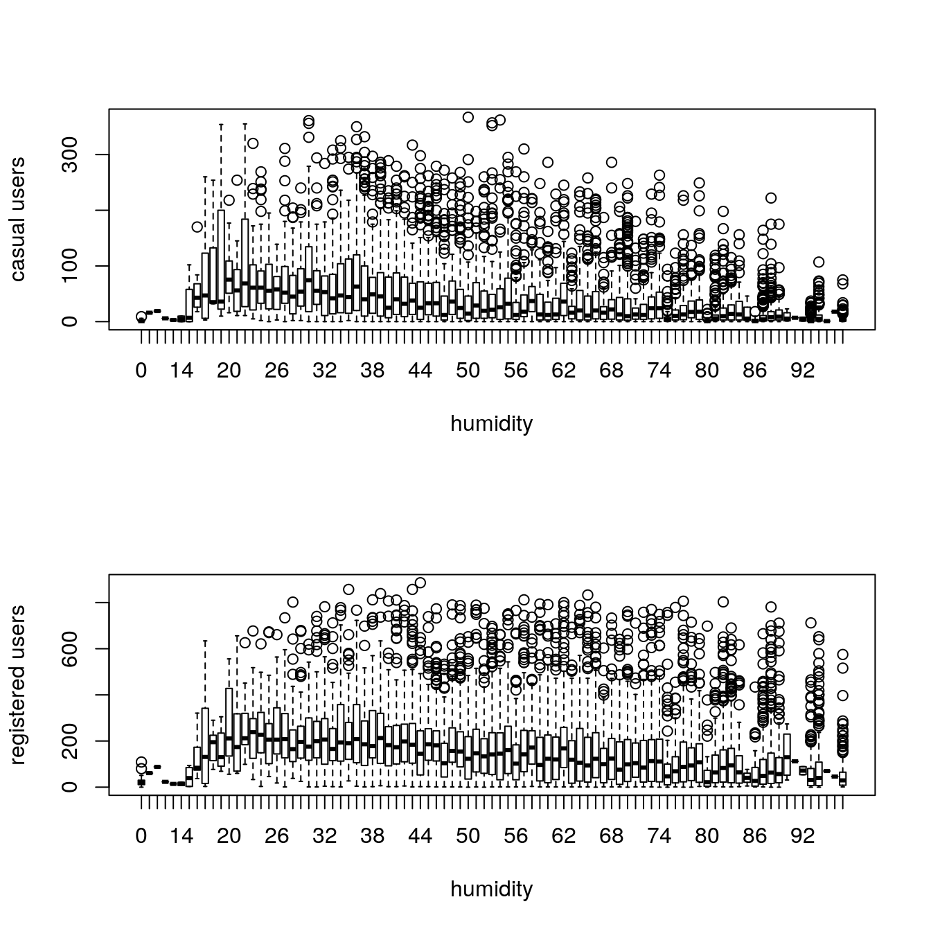
29.4.7 Rain

The demand of bikes will be lower on a rainy day as compared to a sunny day. Similarly, higher humidity will cause to lower the demand and vice versa.

We use the variable weather (1 to 4) to analyze riding under rain conditions.

29.4.7.1 Boxplot of rain effect on bike riding, training set

par(mfrow=c(2,1))
boxplot(train$casual ~ train$weather, xlab="day", ylab="casual users")
boxplot(train$registered ~ train$weather, xlab="day", ylab="registered users")

Registered used tend to ride even with rain.

29.4.8 Temperature

Would high or low temperature encourage or disencourage bike riding?

29.4.8.1 boxplot of temperature effect, training set

par(mfrow=c(2,1))
boxplot(train$casual ~ train$temp, xlab="temp", ylab="casual users")
boxplot(train$registered ~ train$temp, xlab="temp", ylab="registered users")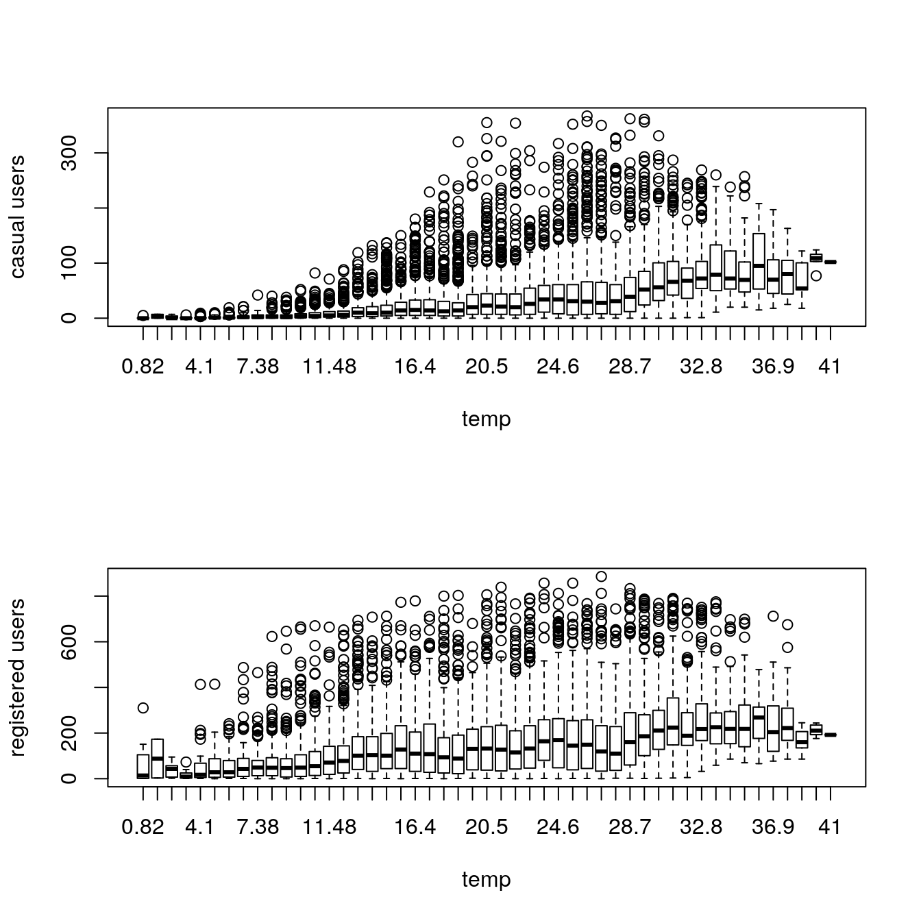

Casual users tend to ride with milder temperatures while registered users ride even at low temperatures.

29.4.9 Correlation

sub = data.frame(train$registered, train$casual, train$count, train$temp,
                 train$humidity, train$atemp, train$windspeed)
cor(sub)
#>                  train.registered train.casual train.count train.temp
#> train.registered           1.0000       0.4972       0.971     0.3186
#> train.casual               0.4972       1.0000       0.690     0.4671
#> train.count                0.9709       0.6904       1.000     0.3945
#> train.temp                 0.3186       0.4671       0.394     1.0000
#> train.humidity            -0.2655      -0.3482      -0.317    -0.0649
#> train.atemp                0.3146       0.4621       0.390     0.9849
#> train.windspeed            0.0911       0.0923       0.101    -0.0179
#>                  train.humidity train.atemp train.windspeed
#> train.registered        -0.2655      0.3146          0.0911
#> train.casual            -0.3482      0.4621          0.0923
#> train.count             -0.3174      0.3898          0.1014
#> train.temp              -0.0649      0.9849         -0.0179
#> train.humidity           1.0000     -0.0435         -0.3186
#> train.atemp             -0.0435      1.0000         -0.0575
#> train.windspeed         -0.3186     -0.0575          1.0000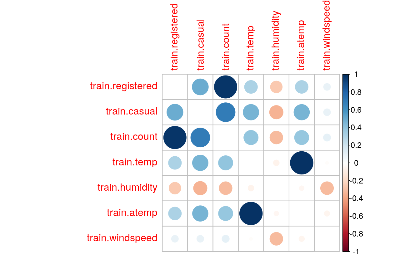

# do not show the diagonal
corrplot(cor(sub), diag = FALSE)

correlation between casual and atemp, temp.
Strong correlation between temp and atemp.

29.4.10 Activity by year

29.4.10.1 Year extraction

# extracting year
data$year = substr(data$datetime, 1, 4)
data$year = as.factor(data$year)

# ignore the division of data again and again, this could have been done together also
train = data[as.integer(substr(data$datetime,9,10)) < 20,]
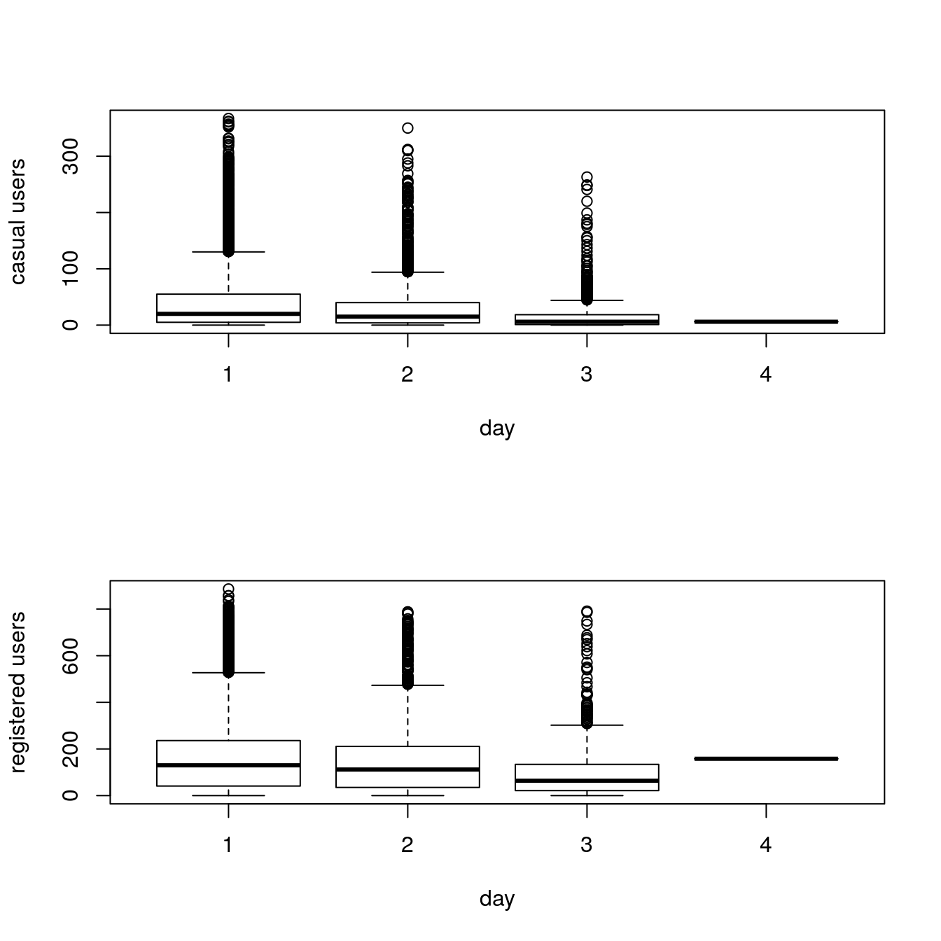
test = data[as.integer(substr(data$datetime,9,10)) > 19,]

29.4.10.2 Trend by year, training set

par(mfrow=c(2,1))
# again some boxplots with different variables
# these boxplots give important information about the dependent variable with respect to the independent variables
boxplot(train$casual ~ train$year, xlab="year", ylab="casual users")
boxplot(train$registered ~ train$year, xlab="year", ylab="registered users")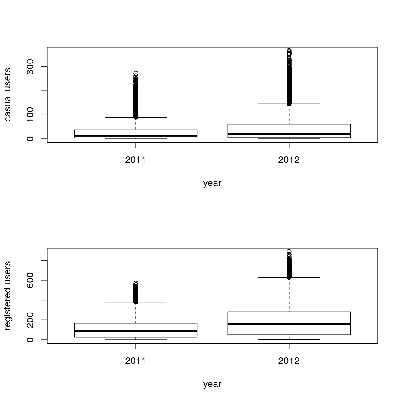

Activity increased in 2012.

29.4.10.3 trend by windspeed, training set

par(mfrow=c(2,1))
boxplot(train$casual ~ train$windspeed, xlab="windspeed", ylab="casual users")
boxplot(train$registered ~ train$windspeed, xlab="windspeed", ylab="registered users")

Casual users ride even with stron winds.

29.4.10.4 trend by humidity, training set

par(mfrow=c(2,1))
boxplot(train$casual ~ train$humidity, xlab="humidity", ylab="casual users")
boxplot(train$registered ~ train$humidity, xlab="humidity", ylab="registered users")

Casual users prefer not to ride with humid weather.

29.5 Feature Engineering

29.5.1 Prepare data

# factoring some variables from integer
data$season     <- as.factor(data$season)
data$weather    <- as.factor(data$weather)
data$holiday    <- as.factor(data$holiday)
data$workingday <- as.factor(data$workingday)

# new column
data$hour <- as.integer(data$hour)

# created this variable to divide a day into parts, but did not finally use it
data$day_part <- 0

# split in training and test sets again
train <- data[as.integer(substr(data$datetime, 9, 10)) < 20,]
test  <- data[as.integer(substr(data$datetime, 9, 10)) > 19,]

# combine the sets
data <- rbind(train, test)

29.5.2 Build hour bins

# for registered users
d = rpart(registered ~ hour, data = train)
fancyRpartPlot(d)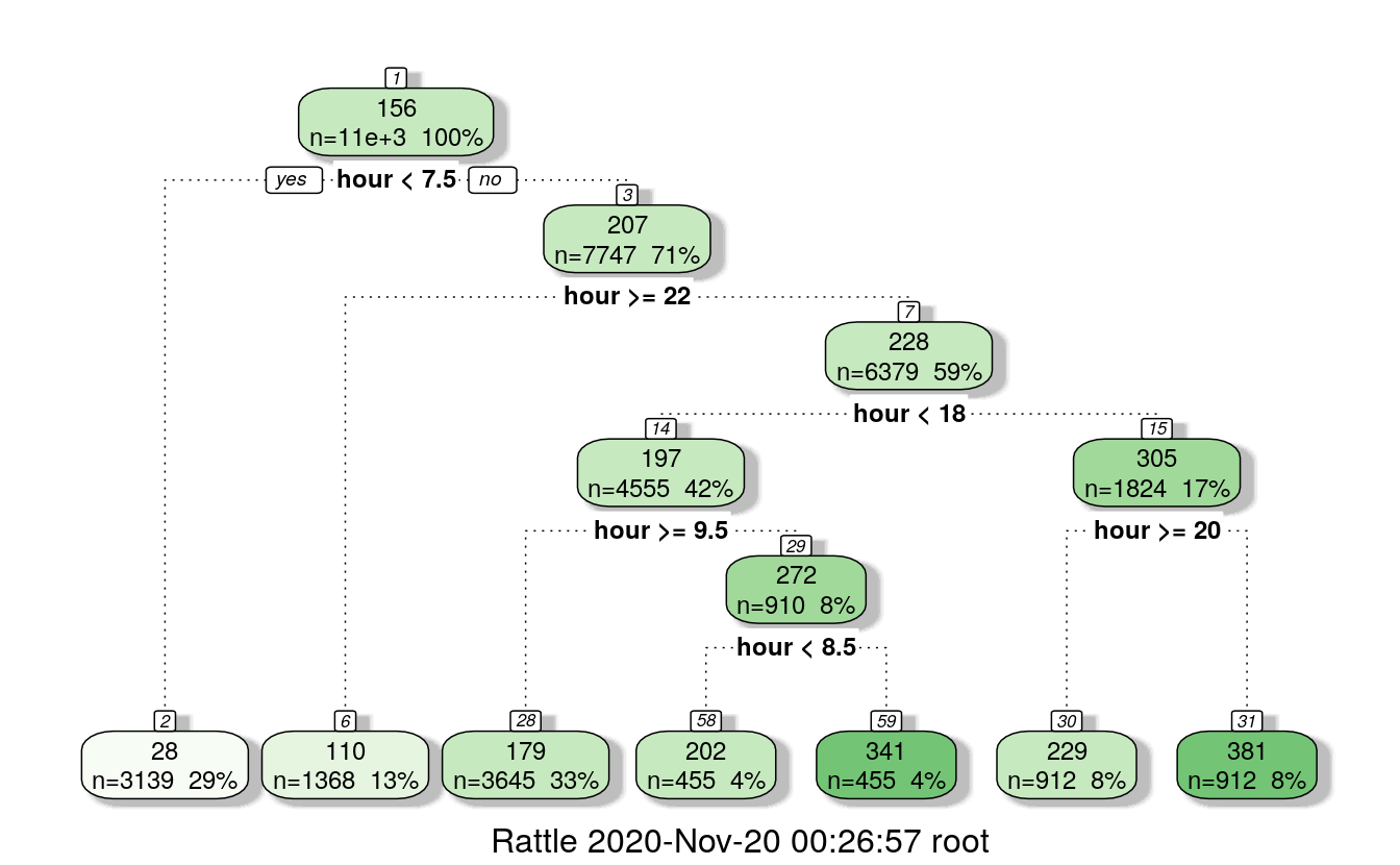

# for casual users
d = rpart(casual ~ hour, data = train)
fancyRpartPlot(d)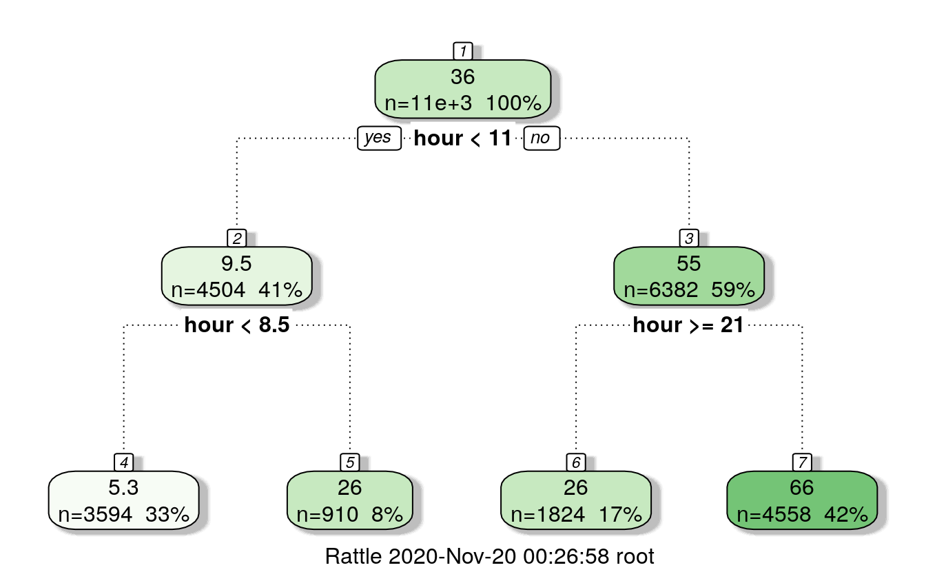

# Assign the timings according to tree
# fill the hour bins
data = rbind(train,test)

# create hour buckets for registered users
# 0,1,2,3,4,5,6,7 < 7.5
# 22,23,24 >=22
# 10,11,12,13,14,15,16,17: h>=9.5 & h<18
# h<9.5 & h<8.5 : 8
# h<9.5 & h>=8.5 : 9
# h>=20: 20,21
# h < 20: 18,19

data$dp_reg = 0
data$dp_reg[data$hour < 8] = 1
data$dp_reg[data$hour >= 22] = 2
data$dp_reg[data$hour > 9 & data$hour < 18] = 3
data$dp_reg[data$hour == 8] = 4
data$dp_reg[data$hour == 9] = 5
data$dp_reg[data$hour == 20 | data$hour == 21] = 6
data$dp_reg[data$hour == 19 | data$hour == 18] = 7

# casual users
# h<11, h<8.5: 0,1,2,3,4,5,6,7,8
# h>=8.5 & h<11: 9, 10 
# h >=11 & h>=21: 21,22,23,24
# h >=11 & h<21: 11,12,13,14,15,16,17,18,19,20
data$dp_cas = 0
data$dp_cas[data$hour < 11 & data$hour >= 8] = 1
data$dp_cas[data$hour == 9 | data$hour == 10] = 2
data$dp_cas[data$hour >= 11 & data$hour < 21] = 3
data$dp_cas[data$hour >= 21] = 4

29.5.3 Temperature bins

# partition the data by temperature, registered users
f = rpart(registered ~ temp, data=train)
fancyRpartPlot(f)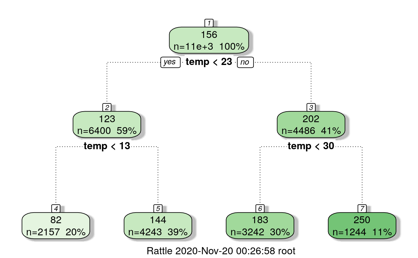

# partition the data by temperature,, casual users
f=rpart(casual ~ temp, data=train)
fancyRpartPlot(f)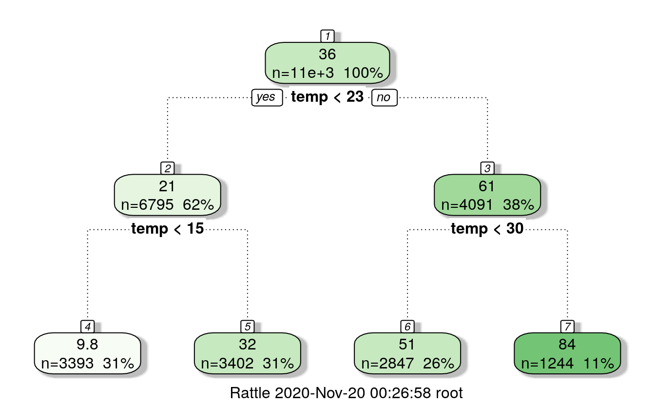

29.5.3.1 Assign temperature ranges accoding to trees

data$temp_reg = 0
data$temp_reg[data$temp < 13] = 1
data$temp_reg[data$temp >= 13 & data$temp < 23] = 2
data$temp_reg[data$temp >= 23 & data$temp < 30] = 3
data$temp_reg[data$temp >= 30] = 4

data$temp_cas = 0
data$temp_cas[data$temp < 15] = 1
data$temp_cas[data$temp >= 15 & data$temp < 23] = 2
data$temp_cas[data$temp >= 23 & data$temp < 30] = 3
data$temp_cas[data$temp >= 30] = 4

29.5.4 Year bins by quarter

# add new variable with the month number
data$month <- substr(data$datetime, 6, 7)
data$month <- as.integer(data$month)

# bin by quarter manually
data$year_part[data$year=='2011']                = 1
data$year_part[data$year=='2011' & data$month>3] = 2
data$year_part[data$year=='2011' & data$month>6] = 3
data$year_part[data$year=='2011' & data$month>9] = 4
data$year_part[data$year=='2012']                = 5
data$year_part[data$year=='2012' & data$month>3] = 6
data$year_part[data$year=='2012' & data$month>6] = 7
data$year_part[data$year=='2012' & data$month>9] = 8
table(data$year_part)
#> 
#>    1    2    3    4    5    6    7    8 
#> 2067 2183 2192 2203 2176 2182 2208 2168

29.5.5 Day Type

Created a variable having categories like “weekday”, “weekend” and “holiday”.

# creating another variable day_type which may affect our accuracy as weekends and weekdays are important in deciding rentals
data$day_type = 0
data$day_type[data$holiday==0 & data$workingday==0] = "weekend"
data$day_type[data$holiday==1]                      = "holiday"
data$day_type[data$holiday==0 & data$workingday==1] = "working day"

# split dataset again
train = data[as.integer(substr(data$datetime,9,10)) < 20,]
test = data[as.integer(substr(data$datetime,9,10)) > 19,]

par(mfrow=c(2,1))
boxplot(train$casual ~ train$dp_cas, xlab = "day partition", ylab="casual users")
boxplot(train$registered ~ train$dp_reg, xlab = "day partition", ylab="registered users")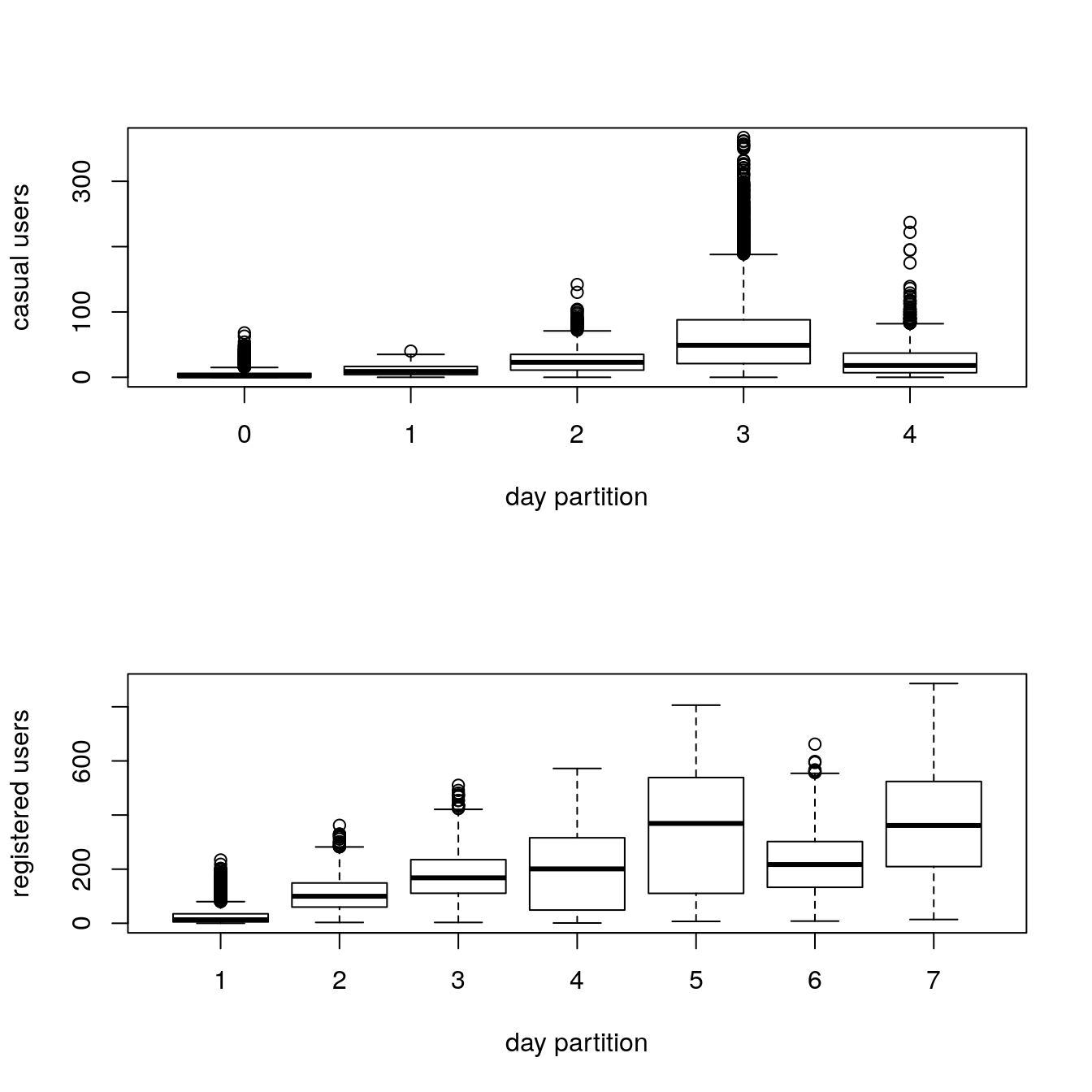

par(mfrow=c(2,1))
boxplot(train$casual ~ train$day_type, xlab = "day type", 
        ylab="casual users", ylim = c(0,900))
boxplot(train$registered ~ train$day_type, xlab = "day type", 
        ylab="registered users", ylim = c(0,900))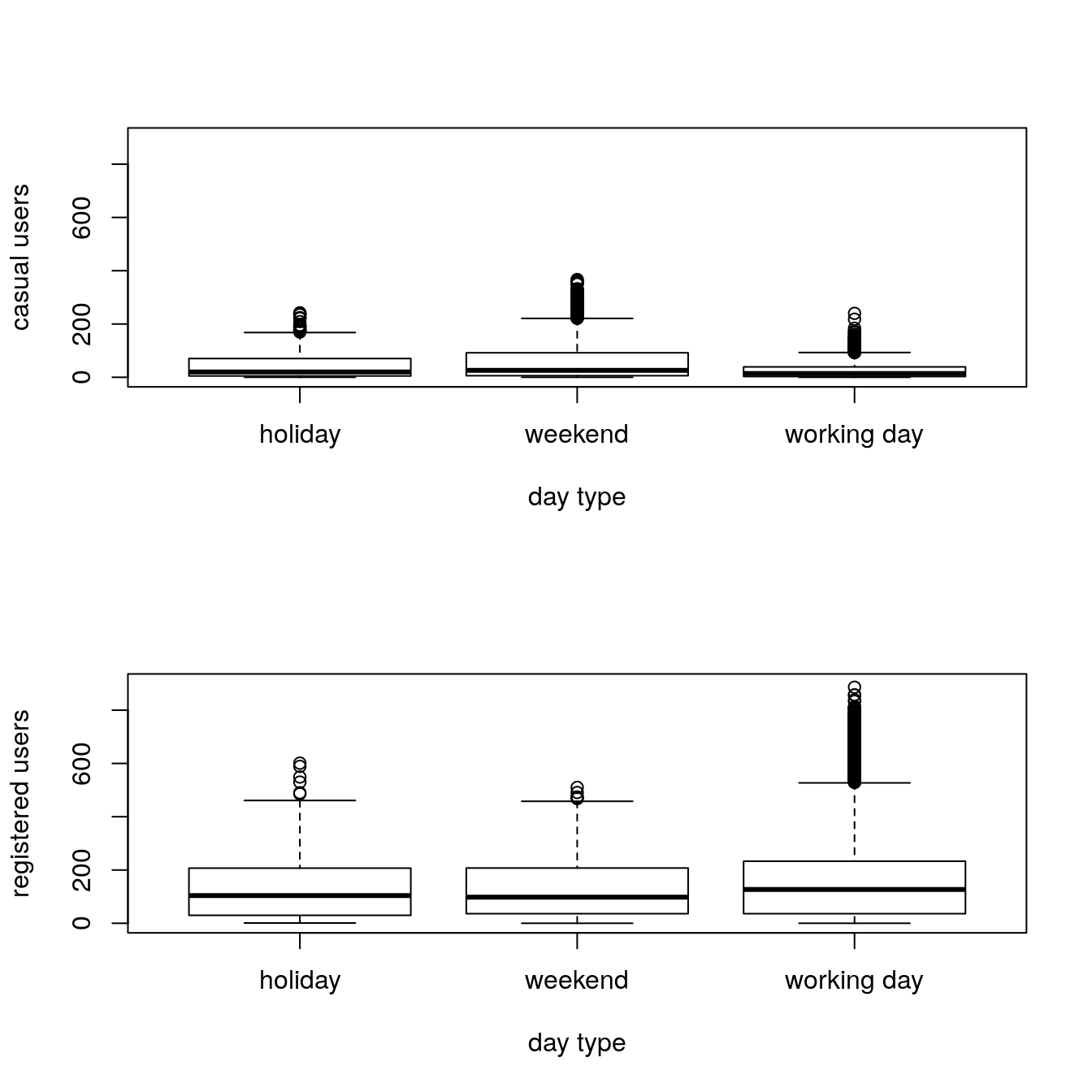

par(mfrow=c(2,1))
boxplot(train$casual ~ train$year_part, xlab = "year partition, quarter", 
        ylab="casual users", ylim = c(0,900))
boxplot(train$registered ~ train$year_part, xlab = "year partition, quarter", 
        ylab="registered users", ylim = c(0,900))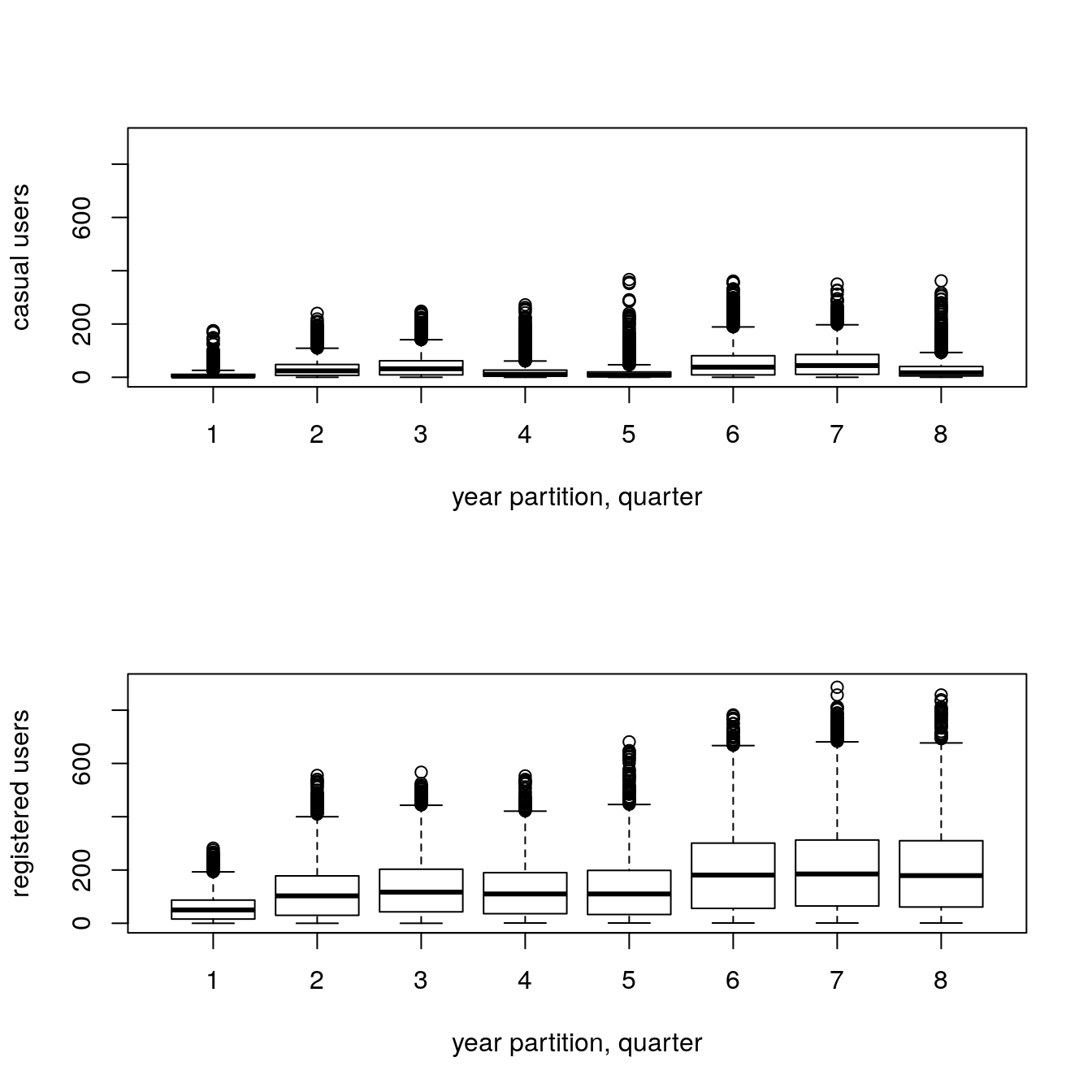

29.5.6 Temperatures

par(mfrow=c(2,1))
boxplot(train$casual ~ train$temp, xlab = "temperature", 
        ylab="casual users", ylim = c(0,900))
boxplot(train$registered ~ train$temp, xlab = "temperature", 
        ylab="registered users", ylim = c(0,900))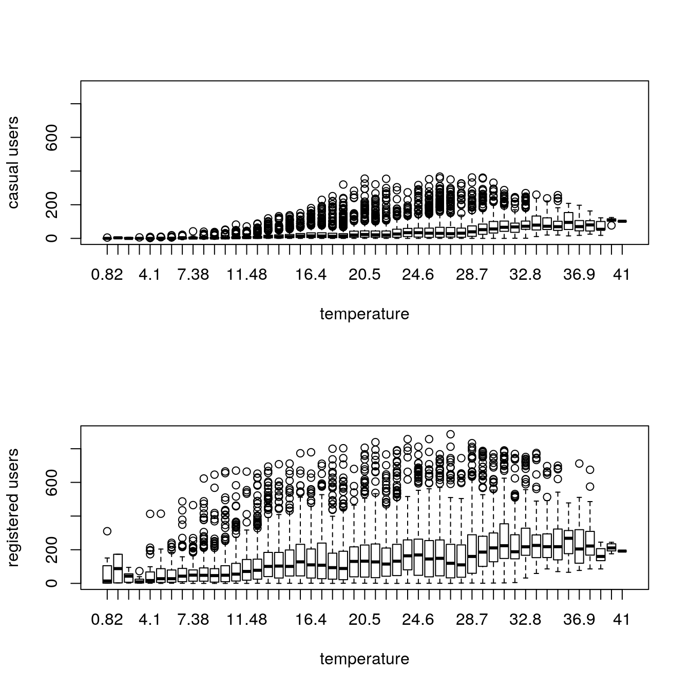

plot(train$temp, train$count)
data <- rbind(train, test)
# data$month <- substr(data$datetime, 6, 7)
# data$month <- as.integer(data$month)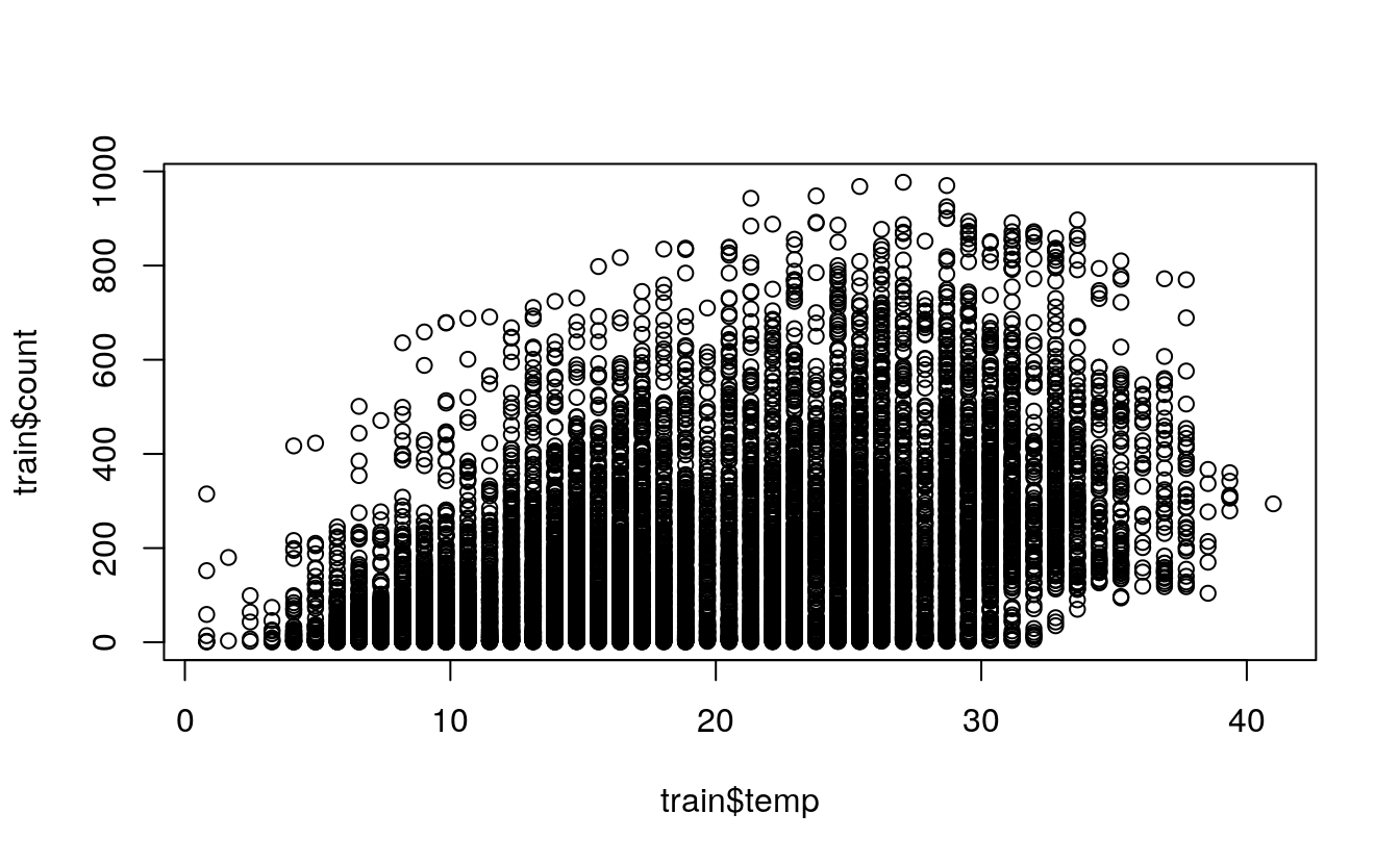

29.5.7 Imputting missing data to wind speed

# dividing total data depending on windspeed to impute/predict the missing values
table(data$windspeed == 0)
#> 
#> FALSE  TRUE 
#> 15199  2180
    # FALSE  TRUE 
    # 15199  2180 

k = data$windspeed == 0

wind_0 = subset(data, k)    # windspeed is zero
wind_1 = subset(data, !k)   # windspeed not zero

tic()
# predicting missing values in windspeed using a random forest model
# this is a different approach to impute missing values rather than 
# just using the mean or median or some other statistic for imputation

set.seed(415)
fit <- randomForest(windspeed ~ season + weather + humidity + month + temp + 
                        year + atemp, 
                    data = wind_1, 
                    importance = TRUE, 
                    ntree = 250)

pred = predict(fit, wind_0)
wind_0$windspeed = pred       # fill with wind speed predictions
toc()
#> 50.787 sec elapsed

# recompose the whole dataset
data = rbind(wind_0, wind_1)

# how many zero values now?
sum(data$windspeed == 0)
#> [1] 0

29.5.8 Weekend variable

Created a separate variable for weekend (0/1)

data$weekend = 0
data$weekend[data$day=="Sunday" | data$day=="Saturday" ] = 1

29.6 Model Building

As this was our first attempt, we applied decision tree, conditional inference tree and random forest algorithms and found that random forest is performing the best. You can also go with regression, boosted regression, neural network and find which one is working well for you.

Before executing the random forest model code, I have followed following steps:

Convert discrete variables into factor (weather, season, hour, holiday, working day, month, day)

str(data)
#> 'data.frame':    17379 obs. of  24 variables:
#>  $ datetime  : Factor w/ 17379 levels "2011-01-01 00:00:00",..: 1 2 3 4 5 7 8 9 10 65 ...
#>  $ season    : Factor w/ 4 levels "1","2","3","4": 1 1 1 1 1 1 1 1 1 1 ...
#>  $ holiday   : Factor w/ 2 levels "0","1": 1 1 1 1 1 1 1 1 1 1 ...
#>  $ workingday: Factor w/ 2 levels "0","1": 1 1 1 1 1 1 1 1 1 2 ...
#>  $ weather   : Factor w/ 4 levels "1","2","3","4": 1 1 1 1 1 1 1 1 1 1 ...
#>  $ temp      : num  9.84 9.02 9.02 9.84 9.84 ...
#>  $ atemp     : num  14.4 13.6 13.6 14.4 14.4 ...
#>  $ humidity  : num  81 80 80 75 75 80 86 75 76 47 ...
#>  $ windspeed : num  9.03 9.05 9.05 9.15 9.15 ...
#>  $ casual    : num  3 8 5 3 0 2 1 1 8 8 ...
#>  $ registered: num  13 32 27 10 1 0 2 7 6 102 ...
#>  $ count     : num  16 40 32 13 1 2 3 8 14 110 ...
#>  $ hour      : int  1 2 3 4 5 7 8 9 10 20 ...
#>  $ day       : chr  "Saturday" "Saturday" "Saturday" "Saturday" ...
#>  $ year      : Factor w/ 2 levels "2011","2012": 1 1 1 1 1 1 1 1 1 1 ...
#>  $ day_part  : num  0 0 0 0 0 0 0 0 0 0 ...
#>  $ dp_reg    : num  1 1 1 1 1 1 4 5 3 6 ...
#>  $ dp_cas    : num  0 0 0 0 0 0 1 2 2 3 ...
#>  $ temp_reg  : num  1 1 1 1 1 1 1 1 2 1 ...
#>  $ temp_cas  : num  1 1 1 1 1 1 1 1 1 1 ...
#>  $ month     : int  1 1 1 1 1 1 1 1 1 1 ...
#>  $ year_part : num  1 1 1 1 1 1 1 1 1 1 ...
#>  $ day_type  : chr  "weekend" "weekend" "weekend" "weekend" ...
#>  $ weekend   : num  1 1 1 1 1 1 1 1 1 0 ...

29.6.1 Convert variables to factors

# converting all relevant categorical variables into factors to feed to our random forest model
data$season     = as.factor(data$season)
data$holiday    = as.factor(data$holiday)
data$workingday = as.factor(data$workingday)
data$weather    = as.factor(data$weather)
data$hour       = as.factor(data$hour)
data$month      = as.factor(data$month)
data$day_part   = as.factor(data$dp_cas)
data$day_type   = as.factor(data$dp_reg)
data$day        = as.factor(data$day)
data$temp_cas   = as.factor(data$temp_cas)
data$temp_reg   = as.factor(data$temp_reg)

str(data)
#> 'data.frame':    17379 obs. of  24 variables:
#>  $ datetime  : Factor w/ 17379 levels "2011-01-01 00:00:00",..: 1 2 3 4 5 7 8 9 10 65 ...
#>  $ season    : Factor w/ 4 levels "1","2","3","4": 1 1 1 1 1 1 1 1 1 1 ...
#>  $ holiday   : Factor w/ 2 levels "0","1": 1 1 1 1 1 1 1 1 1 1 ...
#>  $ workingday: Factor w/ 2 levels "0","1": 1 1 1 1 1 1 1 1 1 2 ...
#>  $ weather   : Factor w/ 4 levels "1","2","3","4": 1 1 1 1 1 1 1 1 1 1 ...
#>  $ temp      : num  9.84 9.02 9.02 9.84 9.84 ...
#>  $ atemp     : num  14.4 13.6 13.6 14.4 14.4 ...
#>  $ humidity  : num  81 80 80 75 75 80 86 75 76 47 ...
#>  $ windspeed : num  9.03 9.05 9.05 9.15 9.15 ...
#>  $ casual    : num  3 8 5 3 0 2 1 1 8 8 ...
#>  $ registered: num  13 32 27 10 1 0 2 7 6 102 ...
#>  $ count     : num  16 40 32 13 1 2 3 8 14 110 ...
#>  $ hour      : Factor w/ 24 levels "1","2","3","4",..: 1 2 3 4 5 7 8 9 10 20 ...
#>  $ day       : Factor w/ 7 levels "Friday","Monday",..: 3 3 3 3 3 3 3 3 3 2 ...
#>  $ year      : Factor w/ 2 levels "2011","2012": 1 1 1 1 1 1 1 1 1 1 ...
#>  $ day_part  : Factor w/ 5 levels "0","1","2","3",..: 1 1 1 1 1 1 2 3 3 4 ...
#>  $ dp_reg    : num  1 1 1 1 1 1 4 5 3 6 ...
#>  $ dp_cas    : num  0 0 0 0 0 0 1 2 2 3 ...
#>  $ temp_reg  : Factor w/ 4 levels "1","2","3","4": 1 1 1 1 1 1 1 1 2 1 ...
#>  $ temp_cas  : Factor w/ 4 levels "1","2","3","4": 1 1 1 1 1 1 1 1 1 1 ...
#>  $ month     : Factor w/ 12 levels "1","2","3","4",..: 1 1 1 1 1 1 1 1 1 1 ...
#>  $ year_part : num  1 1 1 1 1 1 1 1 1 1 ...
#>  $ day_type  : Factor w/ 7 levels "1","2","3","4",..: 1 1 1 1 1 1 4 5 3 6 ...
#>  $ weekend   : num  1 1 1 1 1 1 1 1 1 0 ...

As we know that dependent variables have natural outliers so we will predict log of dependent variables.
Predict bike demand registered and casual users separately. \(y1 = \log(casual+1)\) and \(y2 = \log(registered+1)\), Here we have added 1 to deal with zero values in the casual and registered columns.

# separate again as train and test set
train = data[as.integer(substr(data$datetime, 9, 10)) < 20,]
test = data[as.integer(substr(data$datetime, 9, 10)) > 19,]

29.6.2 Log transform

# log transformation for some skewed variables, 
# which can be seen from their distribution
train$reg1   = train$registered + 1
train$cas1   = train$casual + 1
train$logcas = log(train$cas1)
train$logreg = log(train$reg1)
test$logreg  = 0
test$logcas  = 0

29.6.2.1 Plot by weather, by season

# cartesian plot
par(mfrow=c(2,1))
boxplot(train$registered ~ train$weather, xlab="weather", ylab="registered users")
boxplot(train$registered ~ train$season, xlab="season", ylab="registered users")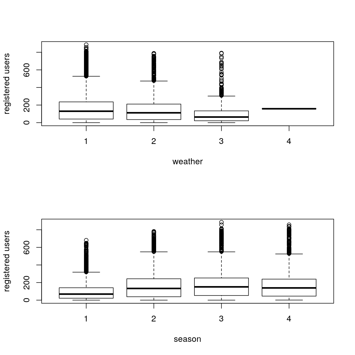

# semilog plot
par(mfrow=c(2,1))
boxplot(train$logreg ~ train$weather, xlab = "weather")
boxplot(train$logreg ~ train$season, xlab = "season")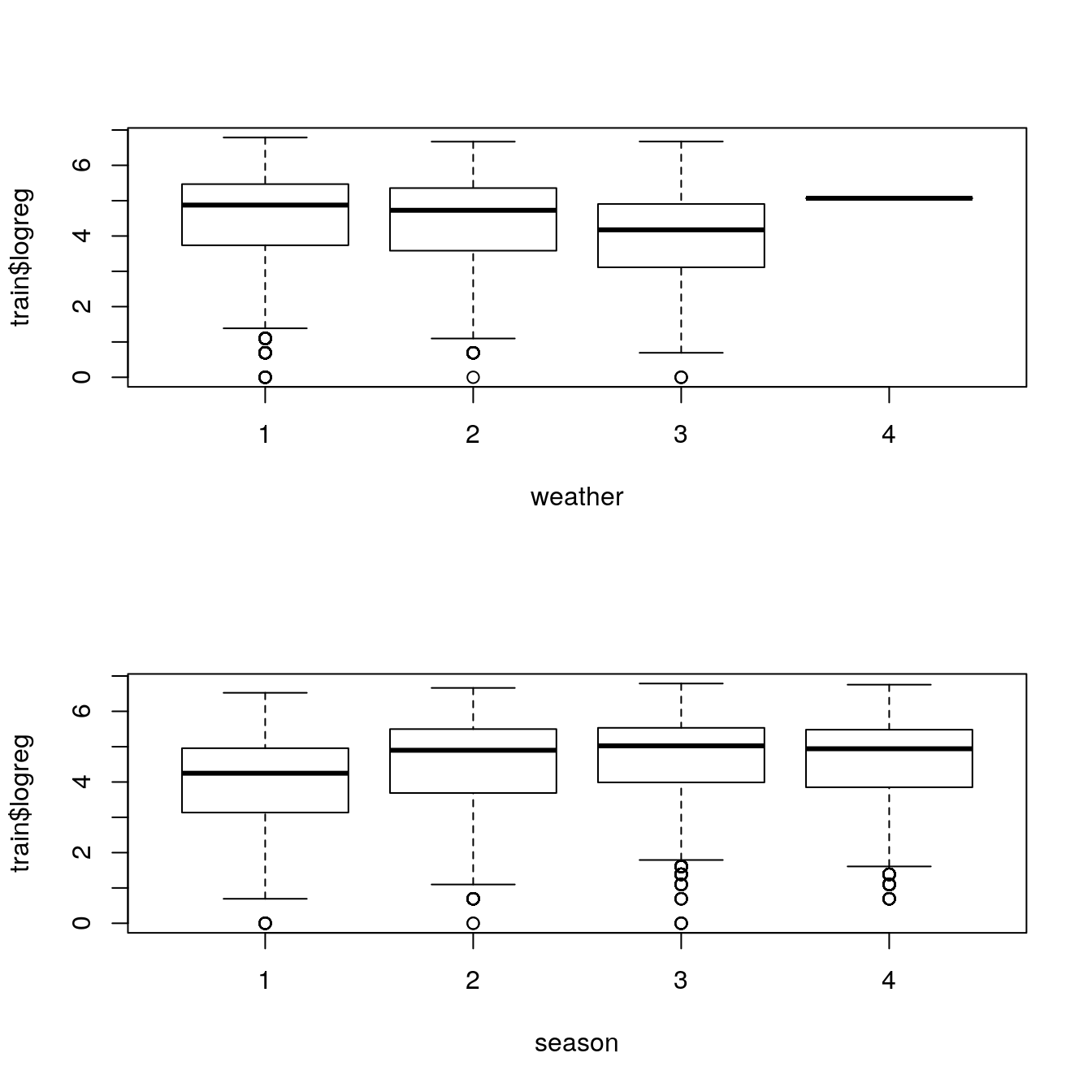

29.6.3 Predicting for registered and casual users, test dataset

tic()
# final model building using random forest
# note that we build different models for predicting for 
# registered and casual users
# this was seen as giving best result after a lot of experimentation
set.seed(415)
fit1 <- randomForest(logreg ~ hour + workingday + day + holiday + day_type +
                         temp_reg + humidity + atemp + windspeed + season + 
                         weather + dp_reg + weekend + year + year_part, 
                     data = train, 
                     importance = TRUE, 
                     ntree = 250)

pred1 = predict(fit1, test)
test$logreg = pred1
toc()
#> 113.34 sec elapsed

# casual users
set.seed(415)
fit2 <- randomForest(logcas ~ hour + day_type + day + humidity + atemp + 
                         temp_cas + windspeed + season + weather + holiday +
                         workingday + dp_cas + weekend + year + year_part, 
                     data = train, importance = TRUE, ntree = 250)

pred2 = predict(fit2, test)
test$logcas = pred2

29.6.4 Preparing and exporting results

# creating the final submission file
# reverse log conversion
test$registered <- exp(test$logreg) - 1
test$casual     <- exp(test$logcas) - 1
test$count      <- test$casual + test$registered

r <- data.frame(datetime = test$datetime, 
                casual = test$casual, 
                registered = test$registered)

print(sum(r$casual))
#> [1] 205804
print(sum(r$registered))
#> [1] 962834

s <- data.frame(datetime = test$datetime, count = test$count)
write.csv(s, file =file.path(data_out_dir, "bike-submit.csv"), row.names = FALSE)

# sum(cas+reg) = 1168638
# month number now is correct

After following the steps mentioned above, you can score 0.38675 on Kaggle leaderboard i.e. top 5 percentile of total participants. As you might have seen, we have not applied any extraordinary science in getting to this level. But, the real competition starts here. I would like to see, if I can improve this further by use of more features and some more advanced modeling techniques.

29.7 End Notes

In this article, we have looked at structured approach of problem solving and how this method can help you to improve performance. I would recommend you to generate hypothesis before you deep dive in the data set as this technique will not limit your thought process. You can improve your performance by applying advanced techniques (or ensemble methods) and understand your data trend better.

You can find the complete solution here : GitHub Link

# this is the older submission. months were incomplete
old <- read.csv(file = file.path(data_raw_dir, "bike-submit-old.csv"))
sum(old$count)
#> [1] 1164829

28 Predicting Flu outcome comparing eight classification algorithms

30 Prediction of arrhythmia with deep neural nets