38 Temperature modeling using nested dataframes

Dataset: temperature.csv

38.1 Introduction

http://ijlyttle.github.io/isugg_purrr/presentation.html#(1)

38.1.1 Packages to run this presentation

library("readr")
library("tibble")
library("dplyr")
library("tidyr")
library("stringr")
library("ggplot2")
library("purrr")
library("broom")

38.1.2 Motivation

As you know, purrr is a recent package from Hadley Wickham, focused on lists and functional programming, like dplyr is focused on data-frames.

I figure a good way to learn a new package is to try to solve a problem, so we have a dataset:

you can view or download
you can download the source of this presentation
these are three temperatures recorded simultaneously in a piece of electronics
it will be very valuable to be able to characterize the transient temperature for each sensor
we want to apply the same set of models across all three sensors
it will be easier to show using pictures

38.2 Prepare the data

38.2.1 Let’s get the data into shape

Using the readr package

temperature_wide <- 
  read_csv(file.path(data_raw_dir, "temperature.csv")) %>%
  print()
#> Parsed with column specification:
#> cols(
#>   instant = col_datetime(format = ""),
#>   temperature_a = col_double(),
#>   temperature_b = col_double(),
#>   temperature_c = col_double()
#> )
#> # A tibble: 327 x 4
#>   instant             temperature_a temperature_b temperature_c
#>   <dttm>                      <dbl>         <dbl>         <dbl>
#> 1 2015-11-13 06:10:19          116.          91.7          84.2
#> 2 2015-11-13 06:10:23          116.          91.7          84.2
#> 3 2015-11-13 06:10:27          116.          91.6          84.2
#> 4 2015-11-13 06:10:31          116.          91.7          84.2
#> 5 2015-11-13 06:10:36          116.          91.7          84.2
#> 6 2015-11-13 06:10:41          116.          91.6          84.2
#> # … with 321 more rows

38.2.2 Is `temperature_wide` “tidy”?

#> # A tibble: 327 x 4
#>   instant             temperature_a temperature_b temperature_c
#>   <dttm>                      <dbl>         <dbl>         <dbl>
#> 1 2015-11-13 06:10:19          116.          91.7          84.2
#> 2 2015-11-13 06:10:23          116.          91.7          84.2
#> 3 2015-11-13 06:10:27          116.          91.6          84.2
#> 4 2015-11-13 06:10:31          116.          91.7          84.2
#> 5 2015-11-13 06:10:36          116.          91.7          84.2
#> 6 2015-11-13 06:10:41          116.          91.6          84.2
#> # … with 321 more rows

Why or why not?

38.2.3 Tidy data

Each column is a variable
Each row is an observation
Each cell is a value

(http://www.jstatsoft.org/v59/i10/paper)

My personal observation is that “tidy” can depend on the context, on what you want to do with the data.

38.2.4 Let’s get this into a tidy form

temperature_tall <-
  temperature_wide %>%
  gather(key = "id_sensor", value = "temperature", starts_with("temp")) %>%
  mutate(id_sensor = str_replace(id_sensor, "temperature_", "")) %>%
  print()
#> # A tibble: 981 x 3
#>   instant             id_sensor temperature
#>   <dttm>              <chr>           <dbl>
#> 1 2015-11-13 06:10:19 a                116.
#> 2 2015-11-13 06:10:23 a                116.
#> 3 2015-11-13 06:10:27 a                116.
#> 4 2015-11-13 06:10:31 a                116.
#> 5 2015-11-13 06:10:36 a                116.
#> 6 2015-11-13 06:10:41 a                116.
#> # … with 975 more rows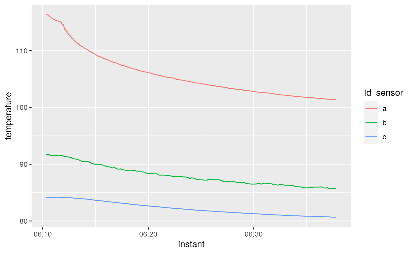

38.2.5 Now, it’s easier to visualize

temperature_tall %>%
  ggplot(aes(x = instant, y = temperature, color = id_sensor)) +
  geom_line()

38.2.6 Calculate delta time (\(\Delta t\)) and delta temperature (\(\Delta T\))

delta_time \(\Delta t\)

change in time since event started, s

delta_temperature: \(\Delta T\)

change in temperature since event started, °C

delta <- 
  temperature_tall %>%
  arrange(id_sensor, instant) %>%
  group_by(id_sensor) %>%
  mutate(
    delta_time = as.numeric(instant) - as.numeric(instant[[1]]),
    delta_temperature = temperature - temperature[[1]]
  ) %>%
  select(id_sensor, delta_time, delta_temperature)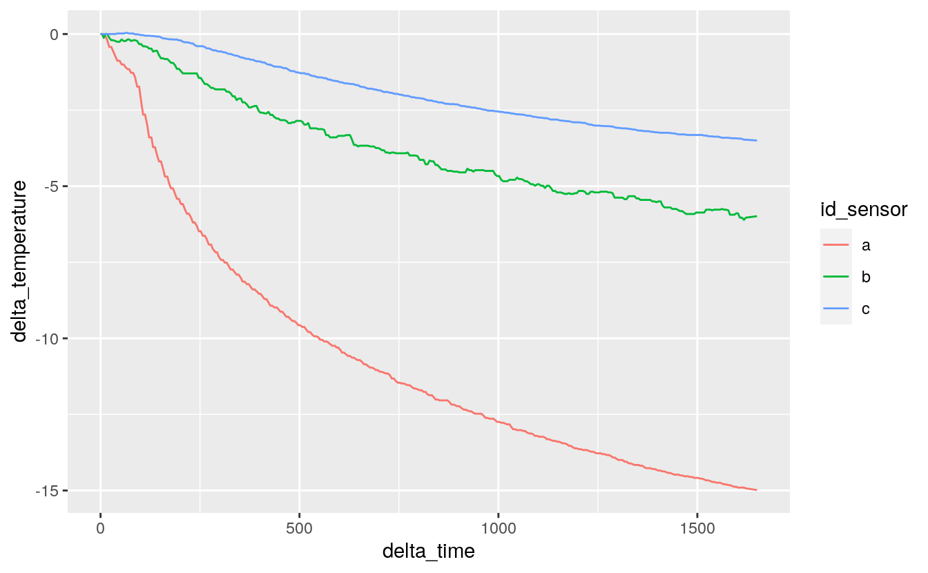

38.2.7 Let’s have a look

# plot delta time vs delta temperature, by sensor
delta %>%
  ggplot(aes(x = delta_time, y = delta_temperature, color = id_sensor)) +
  geom_line()

38.3 Define the models

We want to see how three different curve-fits might perform on these three data-sets:

38.3.0.1 Newtonian cooling

\[\Delta T = \Delta {T_0} * (1 - e^{-\frac{\delta t}{\tau_0}})\]

38.3.1 Semi-infinite solid

\[\Delta T = \Delta T_0 * erfc(\sqrt{\frac{\tau_0}{\delta t}}))\]

38.3.2 Semi-infinite solid with convection

\[\Delta T = \Delta T_0 * \big [ \operatorname erfc(\sqrt{\frac{\tau_0}{\delta t}}) - e^ {Bi_0 + (\frac {Bi_0}{2})^2 \frac {\delta t}{\tau_0}} * \operatorname erfc (\sqrt \frac{\tau_0}{\delta t} + \frac {Bi_0}{2} * \sqrt \frac{\delta t }{\tau_0} \big]\]

38.3.3 `erf` and `erfc` functions

# reference: http://stackoverflow.com/questions/29067916/r-error-function-erfz
# (see Abramowitz and Stegun 29.2.29)
erf <- function(x) 2 * pnorm(x * sqrt(2)) - 1
erfc <- function(x) 2 * pnorm(x * sqrt(2), lower = FALSE)

38.3.4 Newton cooling equation

newton_cooling <- function(x) {
  nls(
    delta_temperature ~ delta_temperature_0 * (1 - exp(-delta_time/tau_0)),
    start = list(delta_temperature_0 = -10, tau_0 = 50),
    data = x
  )
}

38.3.5 Temperature models: simple and convection

semi_infinite_simple <- function(x) {
  nls(
    delta_temperature ~ delta_temperature_0 * erfc(sqrt(tau_0 / delta_time)),
    start = list(delta_temperature_0 = -10, tau_0 = 50),
    data = x
  )    
}

semi_infinite_convection <- function(x){
  nls(
    delta_temperature ~
      delta_temperature_0 * (
        erfc(sqrt(tau_0 / delta_time)) -
        exp(Bi_0 + (Bi_0/2)^2 * delta_time / tau_0) *
          erfc(sqrt(tau_0 / delta_time) + 
        (Bi_0/2) * sqrt(delta_time / tau_0))
      ),
    start = list(delta_temperature_0 = -5, tau_0 = 50, Bi_0 = 1.e6),
    data = x
  )
}

38.4 Test modeling on one dataset

38.4.1 Before going into `purrr`

Before doing anything, we want to show that we can do something with one dataset and one model-function:

# only one sensor; it is a test
tmp_data <- delta %>% filter(id_sensor == "a")

tmp_model <- newton_cooling(tmp_data)

summary(tmp_model)
#> 
#> Formula: delta_temperature ~ delta_temperature_0 * (1 - exp(-delta_time/tau_0))
#> 
#> Parameters:
#>                     Estimate Std. Error t value Pr(>|t|)    
#> delta_temperature_0 -15.0608     0.0526    -286   <2e-16 ***
#> tau_0               500.0138     4.8367     103   <2e-16 ***
#> ---
#> Signif. codes:  0 '***' 0.001 '**' 0.01 '*' 0.05 '.' 0.1 ' ' 1
#> 
#> Residual standard error: 0.327 on 325 degrees of freedom
#> 
#> Number of iterations to convergence: 7 
#> Achieved convergence tolerance: 4.14e-06

38.4.2 Look at predictions

# apply prediction and make it tidy
tmp_pred <- 
  tmp_data %>%
  mutate(modeled = predict(tmp_model, data = .)) %>%
  select(id_sensor, delta_time, measured = delta_temperature, modeled) %>%
  gather("type", "delta_temperature", measured:modeled) %>%
  print()
#> # A tibble: 654 x 4
#> # Groups:   id_sensor [1]
#>   id_sensor delta_time type     delta_temperature
#>   <chr>          <dbl> <chr>                <dbl>
#> 1 a                  0 measured             0    
#> 2 a                  4 measured             0    
#> 3 a                  8 measured            -0.06 
#> 4 a                 12 measured            -0.06 
#> 5 a                 17 measured            -0.211
#> 6 a                 22 measured            -0.423
#> # … with 648 more rows

38.4.3 Plot Newton model

tmp_pred %>%
  ggplot(aes(x = delta_time, y = delta_temperature, linetype = type)) +
  geom_line() +
  labs(title = "Newton temperature model", subtitle = "One sensor: a")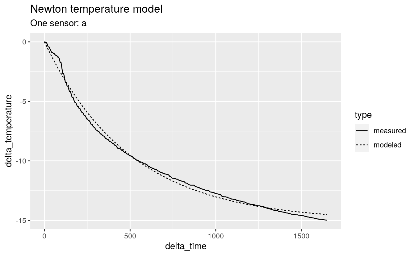

38.4.4 “Regular” data-frame (deltas)

print(delta)
#> # A tibble: 981 x 3
#> # Groups:   id_sensor [3]
#>   id_sensor delta_time delta_temperature
#>   <chr>          <dbl>             <dbl>
#> 1 a                  0             0    
#> 2 a                  4             0    
#> 3 a                  8            -0.06 
#> 4 a                 12            -0.06 
#> 5 a                 17            -0.211
#> 6 a                 22            -0.423
#> # … with 975 more rows

Each column of the dataframe is a vector - in this case, a character vector and two doubles

38.5 Making a nested dataframe

38.5.1 How to make a weird data-frame

Here’s where the fun starts - a column of a data-frame can be a list.

use tidyr::nest() to makes a column data, which is a list of data-frames
this seems like a stronger expression of the dplyr::group_by() idea

# nest delta_time and delta_temperature variables
delta_nested <- 
  delta %>%
  nest(-id_sensor) %>%
  print()
#> Warning: All elements of `...` must be named.
#> Did you want `data = c(delta_time, delta_temperature)`?
#> # A tibble: 3 x 2
#> # Groups:   id_sensor [3]
#>   id_sensor data              
#>   <chr>     <list>            
#> 1 a         <tibble [327 × 2]>
#> 2 b         <tibble [327 × 2]>
#> 3 c         <tibble [327 × 2]>

38.5.2 Map dataframes to a modeling function (Newton)

map() is like lapply()
map() returns a list-column (it keeps the weirdness)

model_nested <-
  delta_nested %>%
  mutate(model = map(data, newton_cooling)) %>%
  print()
#> # A tibble: 3 x 3
#> # Groups:   id_sensor [3]
#>   id_sensor data               model 
#>   <chr>     <list>             <list>
#> 1 a         <tibble [327 × 2]> <nls> 
#> 2 b         <tibble [327 × 2]> <nls> 
#> 3 c         <tibble [327 × 2]> <nls>

We get an additional list-column model.

38.5.3 We can use `map2()` to make the predictions

map2() is like mapply()
designed to map two colunms (model, data) to a function predict()

predict_nested <-
  model_nested %>%
  mutate(pred = map2(model, data, predict)) %>%
  print()
#> # A tibble: 3 x 4
#> # Groups:   id_sensor [3]
#>   id_sensor data               model  pred       
#>   <chr>     <list>             <list> <list>     
#> 1 a         <tibble [327 × 2]> <nls>  <dbl [327]>
#> 2 b         <tibble [327 × 2]> <nls>  <dbl [327]>
#> 3 c         <tibble [327 × 2]> <nls>  <dbl [327]>

Another list-column pred for the prediction results.

38.5.4 We need to get out of the weirdness

use unnest() to get back to a regular data-frame

predict_unnested <- 
  predict_nested %>%
  unnest(data, pred) %>% 
  print()
#> Warning: unnest() has a new interface. See ?unnest for details.
#> Try `df %>% unnest(c(data, pred))`, with `mutate()` if needed
#> # A tibble: 981 x 5
#> # Groups:   id_sensor [3]
#>   id_sensor delta_time delta_temperature model    pred
#>   <chr>          <dbl>             <dbl> <list>  <dbl>
#> 1 a                  0             0     <nls>   0    
#> 2 a                  4             0     <nls>  -0.120
#> 3 a                  8            -0.06  <nls>  -0.239
#> 4 a                 12            -0.06  <nls>  -0.357
#> 5 a                 17            -0.211 <nls>  -0.503
#> 6 a                 22            -0.423 <nls>  -0.648
#> # … with 975 more rows

38.5.5 We can wrangle the predictions

get into a form that makes it easier to plot

predict_tall <- 
  predict_unnested %>%
  rename(modeled = pred, measured = delta_temperature) %>%
  gather("type", "delta_temperature", modeled, measured) %>%
  print()
#> # A tibble: 1,962 x 5
#> # Groups:   id_sensor [3]
#>   id_sensor delta_time model  type    delta_temperature
#>   <chr>          <dbl> <list> <chr>               <dbl>
#> 1 a                  0 <nls>  modeled             0    
#> 2 a                  4 <nls>  modeled            -0.120
#> 3 a                  8 <nls>  modeled            -0.239
#> 4 a                 12 <nls>  modeled            -0.357
#> 5 a                 17 <nls>  modeled            -0.503
#> 6 a                 22 <nls>  modeled            -0.648
#> # … with 1,956 more rows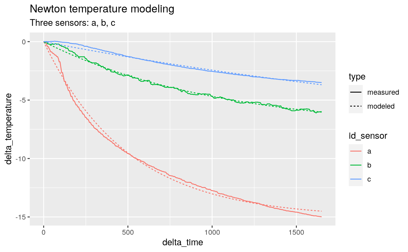

38.5.6 We can visualize the predictions

predict_tall %>%
  ggplot(aes(x = delta_time, y = delta_temperature)) +
  geom_line(aes(color = id_sensor, linetype = type)) +
  labs(title = "Newton temperature modeling", 
       subtitle = "Three sensors: a, b, c")

38.6 Apply multiple models on a nested structure

38.6.1 Step 1: Selection of models

Make a list of functions to model:

list_model <-
  list(
    newton_cooling = newton_cooling,
    semi_infinite_simple = semi_infinite_simple,
    semi_infinite_convection = semi_infinite_convection
  )

38.6.2 Step 2: write a function to define the “inner” loop

# add additional variable with the model name

fn_model <- function(.model, df) {
  # one parameter for the model in the list, the second for the data
  # safer to avoid non-standard evaluation
  # df %>% mutate(model = map(data, .model)) 
  
  df$model <- map(df$data, possibly(.model, NULL))
  df
}

for a given model-function and a given (weird) data-frame, return a modified version of that data-frame with a column model, which is the model-function applied to each element of the data-frame’s data column (which is itself a list of data-frames)
the purrr functions safely() and possibly() are very interesting. I think they could be useful outside of purrr as a friendlier way to do error-handling.

38.6.3 Step 3: Use `map_df()` to define the “outer” loop

# this dataframe will be the second input of fn_model
delta_nested %>% 
  print()
#> # A tibble: 3 x 2
#> # Groups:   id_sensor [3]
#>   id_sensor data              
#>   <chr>     <list>            
#> 1 a         <tibble [327 × 2]>
#> 2 b         <tibble [327 × 2]>
#> 3 c         <tibble [327 × 2]>

# fn_model is receiving two inputs: one from list_model and from delta_nested
model_nested_new <-
  list_model %>%
  map_df(fn_model, delta_nested, .id = "id_model") %>%
  print()
#> # A tibble: 9 x 4
#> # Groups:   id_sensor [3]
#>   id_model             id_sensor data               model 
#>   <chr>                <chr>     <list>             <list>
#> 1 newton_cooling       a         <tibble [327 × 2]> <nls> 
#> 2 newton_cooling       b         <tibble [327 × 2]> <nls> 
#> 3 newton_cooling       c         <tibble [327 × 2]> <nls> 
#> 4 semi_infinite_simple a         <tibble [327 × 2]> <nls> 
#> 5 semi_infinite_simple b         <tibble [327 × 2]> <nls> 
#> 6 semi_infinite_simple c         <tibble [327 × 2]> <nls> 
#> # … with 3 more rows

for each element of a list of model-functions, run the inner-loop function, and row-bind the results into a data-frame
we want to discard the rows where the model failed
we also want to investigate why they failed, but that’s a different talk

38.6.4 Step 4: Use `map()` to identify the null models

model_nested_new <-
  list_model %>%
  map_df(fn_model, delta_nested, .id = "id_model") %>%
  mutate(is_null = map(model, is.null)) %>%
  print()
#> # A tibble: 9 x 5
#> # Groups:   id_sensor [3]
#>   id_model             id_sensor data               model  is_null  
#>   <chr>                <chr>     <list>             <list> <list>   
#> 1 newton_cooling       a         <tibble [327 × 2]> <nls>  <lgl [1]>
#> 2 newton_cooling       b         <tibble [327 × 2]> <nls>  <lgl [1]>
#> 3 newton_cooling       c         <tibble [327 × 2]> <nls>  <lgl [1]>
#> 4 semi_infinite_simple a         <tibble [327 × 2]> <nls>  <lgl [1]>
#> 5 semi_infinite_simple b         <tibble [327 × 2]> <nls>  <lgl [1]>
#> 6 semi_infinite_simple c         <tibble [327 × 2]> <nls>  <lgl [1]>
#> # … with 3 more rows

using map(model, is.null) returns a list column
to use filter(), we have to escape the weirdness

38.6.5 Step 5: `map_lgl()` to identify nulls and get out of the weirdness

model_nested_new <-
  list_model %>%
  map_df(fn_model, delta_nested, .id = "id_model") %>%
  mutate(is_null = map_lgl(model, is.null)) %>%
  print()
#> # A tibble: 9 x 5
#> # Groups:   id_sensor [3]
#>   id_model             id_sensor data               model  is_null
#>   <chr>                <chr>     <list>             <list> <lgl>  
#> 1 newton_cooling       a         <tibble [327 × 2]> <nls>  FALSE  
#> 2 newton_cooling       b         <tibble [327 × 2]> <nls>  FALSE  
#> 3 newton_cooling       c         <tibble [327 × 2]> <nls>  FALSE  
#> 4 semi_infinite_simple a         <tibble [327 × 2]> <nls>  FALSE  
#> 5 semi_infinite_simple b         <tibble [327 × 2]> <nls>  FALSE  
#> 6 semi_infinite_simple c         <tibble [327 × 2]> <nls>  FALSE  
#> # … with 3 more rows

using map_lgl(model, is.null) returns a vector column

38.6.6 Step 6: `filter()` nulls and `select()` variables to clean up

model_nested_new <-
  list_model %>%
  map_df(fn_model, delta_nested, .id = "id_model") %>%
  mutate(is_null = map_lgl(model, is.null)) %>%
  filter(!is_null) %>%
  select(-is_null) %>%
  print()
#> # A tibble: 6 x 4
#> # Groups:   id_sensor [3]
#>   id_model             id_sensor data               model 
#>   <chr>                <chr>     <list>             <list>
#> 1 newton_cooling       a         <tibble [327 × 2]> <nls> 
#> 2 newton_cooling       b         <tibble [327 × 2]> <nls> 
#> 3 newton_cooling       c         <tibble [327 × 2]> <nls> 
#> 4 semi_infinite_simple a         <tibble [327 × 2]> <nls> 
#> 5 semi_infinite_simple b         <tibble [327 × 2]> <nls> 
#> 6 semi_infinite_simple c         <tibble [327 × 2]> <nls>

38.6.7 Step 7: Calculate predictions on nested dataframe

predict_nested <- 
  model_nested_new %>%
  mutate(pred = map2(model, data, predict)) %>%
  print()
#> # A tibble: 6 x 5
#> # Groups:   id_sensor [3]
#>   id_model             id_sensor data               model  pred       
#>   <chr>                <chr>     <list>             <list> <list>     
#> 1 newton_cooling       a         <tibble [327 × 2]> <nls>  <dbl [327]>
#> 2 newton_cooling       b         <tibble [327 × 2]> <nls>  <dbl [327]>
#> 3 newton_cooling       c         <tibble [327 × 2]> <nls>  <dbl [327]>
#> 4 semi_infinite_simple a         <tibble [327 × 2]> <nls>  <dbl [327]>
#> 5 semi_infinite_simple b         <tibble [327 × 2]> <nls>  <dbl [327]>
#> 6 semi_infinite_simple c         <tibble [327 × 2]> <nls>  <dbl [327]>

38.6.8 `unnest()`, make it tall and tidy

predict_tall <-
  predict_nested %>%
  unnest(data, pred) %>% 
  rename(modeled = pred, measured = delta_temperature) %>%
  gather("type", "delta_temperature", modeled, measured) %>%
  print()
#> Warning: unnest() has a new interface. See ?unnest for details.
#> Try `df %>% unnest(c(data, pred))`, with `mutate()` if needed
#> # A tibble: 3,924 x 6
#> # Groups:   id_sensor [3]
#>   id_model       id_sensor delta_time model  type    delta_temperature
#>   <chr>          <chr>          <dbl> <list> <chr>               <dbl>
#> 1 newton_cooling a                  0 <nls>  modeled             0    
#> 2 newton_cooling a                  4 <nls>  modeled            -0.120
#> 3 newton_cooling a                  8 <nls>  modeled            -0.239
#> 4 newton_cooling a                 12 <nls>  modeled            -0.357
#> 5 newton_cooling a                 17 <nls>  modeled            -0.503
#> 6 newton_cooling a                 22 <nls>  modeled            -0.648
#> # … with 3,918 more rows

38.6.9 Visualize the predictions

predict_tall %>%
  ggplot(aes(x = delta_time, y = delta_temperature)) +
  geom_line(aes(color = id_sensor, linetype = type)) +
  facet_grid(id_model ~ .) +
  labs(title = "Newton and Semi-infinite temperature modeling", 
       subtitle = "Three sensors: a, b, c")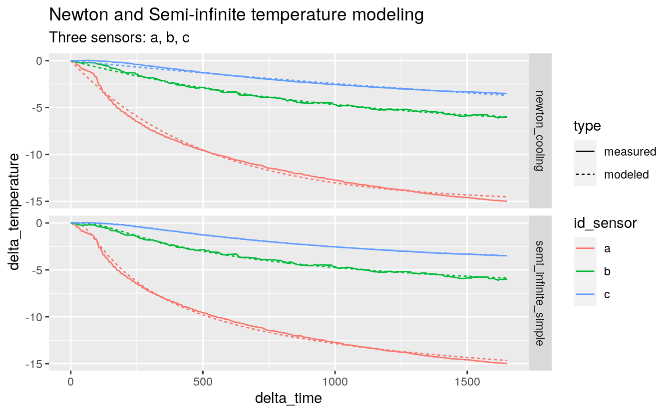

38.6.10 Let’s get the residuals

resid <-
  model_nested_new %>%
  mutate(resid = map(model, resid)) %>%
  unnest(data, resid) %>%
  print()
#> Warning: unnest() has a new interface. See ?unnest for details.
#> Try `df %>% unnest(c(data, resid))`, with `mutate()` if needed
#> # A tibble: 1,962 x 6
#> # Groups:   id_sensor [3]
#>   id_model       id_sensor delta_time delta_temperature model  resid
#>   <chr>          <chr>          <dbl>             <dbl> <list> <dbl>
#> 1 newton_cooling a                  0             0     <nls>  0    
#> 2 newton_cooling a                  4             0     <nls>  0.120
#> 3 newton_cooling a                  8            -0.06  <nls>  0.179
#> 4 newton_cooling a                 12            -0.06  <nls>  0.297
#> 5 newton_cooling a                 17            -0.211 <nls>  0.292
#> 6 newton_cooling a                 22            -0.423 <nls>  0.225
#> # … with 1,956 more rows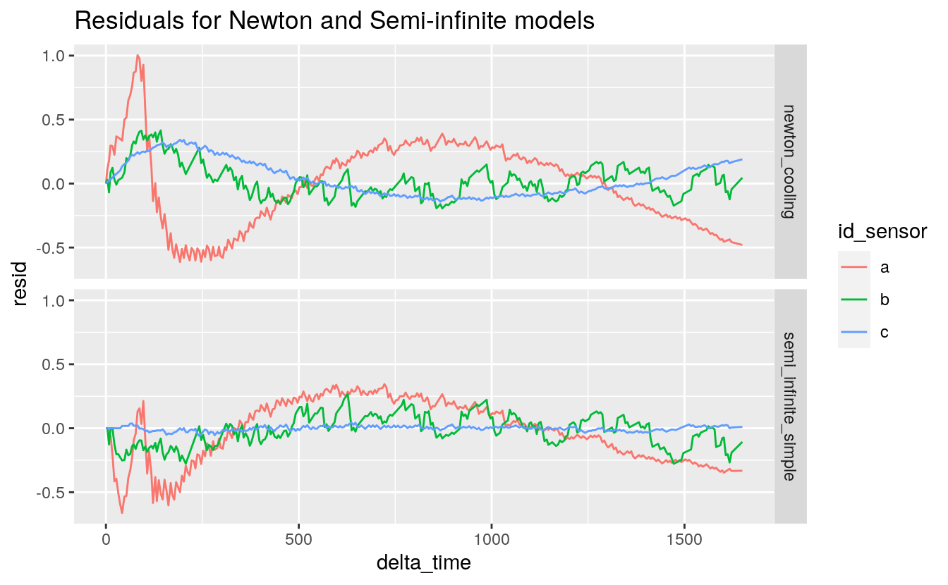

38.6.11 And visualize them

resid %>%
  ggplot(aes(x = delta_time, y = resid)) +
  geom_line(aes(color = id_sensor)) +
  facet_grid(id_model ~ .) +
  labs(title = "Residuals for Newton and Semi-infinite models")

38.7 Using broom package to look at model-statistics

We will use a previous defined dataframe with the model and data:

model_nested_new %>% 
  print()
#> # A tibble: 6 x 4
#> # Groups:   id_sensor [3]
#>   id_model             id_sensor data               model 
#>   <chr>                <chr>     <list>             <list>
#> 1 newton_cooling       a         <tibble [327 × 2]> <nls> 
#> 2 newton_cooling       b         <tibble [327 × 2]> <nls> 
#> 3 newton_cooling       c         <tibble [327 × 2]> <nls> 
#> 4 semi_infinite_simple a         <tibble [327 × 2]> <nls> 
#> 5 semi_infinite_simple b         <tibble [327 × 2]> <nls> 
#> 6 semi_infinite_simple c         <tibble [327 × 2]> <nls>

The tidy() function extracts statistics from a model.

# apply over model_nested_new but only three variables
model_parameters <- 
  model_nested_new %>%
  select(id_model, id_sensor, model) %>%
  mutate(tidy = map(model, tidy)) %>%
  select(-model) %>%
  unnest() %>%
  print()
#> Warning: `cols` is now required.
#> Please use `cols = c(tidy)`
#> # A tibble: 12 x 7
#> # Groups:   id_sensor [3]
#>   id_model      id_sensor term            estimate std.error statistic   p.value
#>   <chr>         <chr>     <chr>              <dbl>     <dbl>     <dbl>     <dbl>
#> 1 newton_cooli… a         delta_temperat…   -15.1     0.0526    -286.  0.       
#> 2 newton_cooli… a         tau_0             500.      4.84       103.  1.07e-250
#> 3 newton_cooli… b         delta_temperat…    -7.59    0.0676    -112.  6.38e-262
#> 4 newton_cooli… b         tau_0            1041.     16.2         64.2 9.05e-187
#> 5 newton_cooli… c         delta_temperat…    -9.87    0.704      -14.0 3.16e- 35
#> 6 newton_cooli… c         tau_0            3525.    299.          11.8 5.61e- 27
#> # … with 6 more rows

38.7.1 Get a sense of the coefficients

model_summary <-
  model_parameters %>%
  select(id_model, id_sensor, term, estimate) %>%
  spread(key = "term", value = "estimate") %>%
  print()
#> # A tibble: 6 x 4
#> # Groups:   id_sensor [3]
#>   id_model             id_sensor delta_temperature_0 tau_0
#>   <chr>                <chr>                   <dbl> <dbl>
#> 1 newton_cooling       a                      -15.1   500.
#> 2 newton_cooling       b                       -7.59 1041.
#> 3 newton_cooling       c                       -9.87 3525.
#> 4 semi_infinite_simple a                      -21.5   139.
#> 5 semi_infinite_simple b                      -10.6   287.
#> 6 semi_infinite_simple c                       -8.04  500.

38.7.2 Summary

this is just a smalll part of purrr
there seem to be parallels between tidyr::nest()/purrr::map() and dplyr::group_by()/dplyr::do()
- to my mind, the purrr framework is more understandable
- update tweet from Hadley

References from Hadley:

37 Comparing Multiple Regression vs a Neural Network

39 Credit Scoring with neuralnet