25 Vehicles classiification with Decision Trees
- Datasets: Vehicle (mlbench)
- Algorithms:
- Decision Trees
- Instructions: book “Applied Predictive Modeling Techniques”, Lewis, N.D.
25.1 Load packages
library(tree)
library(mlbench)

data(Vehicle)
str(Vehicle)
#> 'data.frame':    846 obs. of  19 variables:
#>  $ Comp        : num  95 91 104 93 85 107 97 90 86 93 ...
#>  $ Circ        : num  48 41 50 41 44 57 43 43 34 44 ...
#>  $ D.Circ      : num  83 84 106 82 70 106 73 66 62 98 ...
#>  $ Rad.Ra      : num  178 141 209 159 205 172 173 157 140 197 ...
#>  $ Pr.Axis.Ra  : num  72 57 66 63 103 50 65 65 61 62 ...
#>  $ Max.L.Ra    : num  10 9 10 9 52 6 6 9 7 11 ...
#>  $ Scat.Ra     : num  162 149 207 144 149 255 153 137 122 183 ...
#>  $ Elong       : num  42 45 32 46 45 26 42 48 54 36 ...
#>  $ Pr.Axis.Rect: num  20 19 23 19 19 28 19 18 17 22 ...
#>  $ Max.L.Rect  : num  159 143 158 143 144 169 143 146 127 146 ...
#>  $ Sc.Var.Maxis: num  176 170 223 160 241 280 176 162 141 202 ...
#>  $ Sc.Var.maxis: num  379 330 635 309 325 957 361 281 223 505 ...
#>  $ Ra.Gyr      : num  184 158 220 127 188 264 172 164 112 152 ...
#>  $ Skew.Maxis  : num  70 72 73 63 127 85 66 67 64 64 ...
#>  $ Skew.maxis  : num  6 9 14 6 9 5 13 3 2 4 ...
#>  $ Kurt.maxis  : num  16 14 9 10 11 9 1 3 14 14 ...
#>  $ Kurt.Maxis  : num  187 189 188 199 180 181 200 193 200 195 ...
#>  $ Holl.Ra     : num  197 199 196 207 183 183 204 202 208 204 ...
#>  $ Class       : Factor w/ 4 levels "bus","opel","saab",..: 4 4 3 4 1 1 1 4 4 3 ...
summary(Vehicle[1])
#>       Comp
#>  Min.   : 73.0
#>  1st Qu.: 87.0
#>  Median : 93.0
#>  Mean   : 93.7
#>  3rd Qu.:100.0
#>  Max.   :119.0
summary(Vehicle[2])
#>       Circ
#>  Min.   :33.0
#>  1st Qu.:40.0
#>  Median :44.0
#>  Mean   :44.9
#>  3rd Qu.:49.0
#>  Max.   :59.0
attributes(Vehicle$Class)
#> $levels
#> [1] "bus"  "opel" "saab" "van"
#>
#> $class
#> [1] "factor"25.3 Estimate the decision tree
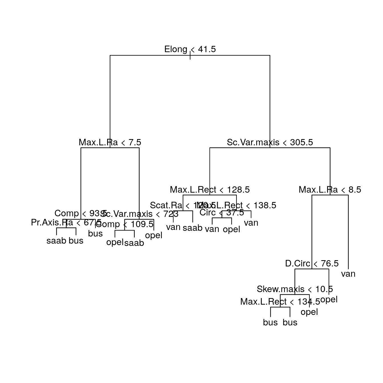
fit <- tree(Class ~., data = trainset, split = "deviance")
fit
#> node), split, n, deviance, yval, (yprob)
#>       * denotes terminal node
#>
#>   1) root 500 1000 opel ( 0 0 0 0 )
#>     2) Elong < 41.5 215  500 saab ( 0 0 0 0 )
#>       4) Max.L.Ra < 7.5 51   50 bus ( 1 0 0 0 )
#>         8) Comp < 93.5 12   20 bus ( 0 0 0 0 )
#>          16) Pr.Axis.Ra < 67.5 7    8 saab ( 0 0 1 0 ) *
#>          17) Pr.Axis.Ra > 67.5 5    0 bus ( 1 0 0 0 ) *
#>         9) Comp > 93.5 39    9 bus ( 1 0 0 0 ) *
#>       5) Max.L.Ra > 7.5 164  200 opel ( 0 1 0 0 )
#>        10) Sc.Var.maxis < 723 149  200 saab ( 0 0 1 0 )
#>          20) Comp < 109.5 137  200 opel ( 0 1 0 0 ) *
#>          21) Comp > 109.5 12    0 saab ( 0 0 1 0 ) *
#>        11) Sc.Var.maxis > 723 15    7 opel ( 0 1 0 0 ) *
#>     3) Elong > 41.5 285  700 van ( 0 0 0 0 )
#>       6) Sc.Var.maxis < 305.5 116  200 van ( 0 0 0 1 )
#>        12) Max.L.Rect < 128.5 40   90 saab ( 0 0 0 0 )
#>          24) Scat.Ra < 120.5 15   30 van ( 0 0 0 1 ) *
#>          25) Scat.Ra > 120.5 25   30 saab ( 0 0 1 0 ) *
#>        13) Max.L.Rect > 128.5 76   90 van ( 0 0 0 1 )
#>          26) Max.L.Rect < 138.5 38   60 van ( 0 0 0 1 )
#>            52) Circ < 37.5 17   10 van ( 0 0 0 1 ) *
#>            53) Circ > 37.5 21   40 opel ( 0 0 0 0 ) *
#>          27) Max.L.Rect > 138.5 38   20 van ( 0 0 0 1 ) *
#>       7) Sc.Var.maxis > 305.5 169  400 bus ( 0 0 0 0 )
#>        14) Max.L.Ra < 8.5 116  200 bus ( 1 0 0 0 )
#>          28) D.Circ < 76.5 97  100 bus ( 1 0 0 0 )
#>            56) Skew.maxis < 10.5 87   70 bus ( 1 0 0 0 )
#>             112) Max.L.Rect < 134.5 12   20 bus ( 0 0 0 0 ) *
#>             113) Max.L.Rect > 134.5 75   20 bus ( 1 0 0 0 ) *
#>            57) Skew.maxis > 10.5 10   20 opel ( 0 0 0 0 ) *
#>          29) D.Circ > 76.5 19   30 opel ( 0 1 0 0 ) *
#>        15) Max.L.Ra > 8.5 53   20 van ( 0 0 0 1 ) *
# fit <- tree(Class ~., data = Vehicle[train,], split ="deviance")
# fit
We use deviance as the splitting criteria, a common alternative is to use split=“gini”.
At each branch of the tree (after root) we see in order: 1. The branch number (e.g. in this case 1,2,14 and 15); 2. the split (e.g. Elong < 41.5); 3. the number of samples going along that split (e.g. 229); 4. the deviance associated with that split (e.g. 489.1); 5. the predicted class (e.g. opel); 6. the associated probabilities (e.g. ( 0.222707 0.410480 0.366812 0.000000 ); 7. and for a terminal node (or leaf), the symbol "*".
summary(fit)
#>
#> Classification tree:
#> tree(formula = Class ~ ., data = trainset, split = "deviance")
#> Variables actually used in tree construction:
#>  [1] "Elong"        "Max.L.Ra"     "Comp"         "Pr.Axis.Ra"   "Sc.Var.maxis"
#>  [6] "Max.L.Rect"   "Scat.Ra"      "Circ"         "D.Circ"       "Skew.maxis"
#> Number of terminal nodes:  16
#> Residual mean deviance:  0.943 = 456 / 484
#> Misclassification error rate: 0.252 = 126 / 500
Notice that summary(fit) shows: 1. The type of tree, in this case a Classification tree; 2. the formula used to fit the tree; 3. the variables used to fit the tree; 4. the number of terminal nodes in this case 15; 5. the residual mean deviance - 0.9381; 6. the misclassification error rate 0.232 or 23.2%.
25.4 Assess model
Unfortunately, classification trees have a tendency to overfit the data. One
approach to reduce this risk is to use cross-validation. For each hold out
sample we fit the model and note at what level the tree gives the best results
(using deviance or the misclassification rate). Then we hold out a different
sample and repeat. This can be carried out using the cv.tree() function.
We use a leave-one-out cross-validation using the misclassification rate and
deviance (FUN=prune.misclass, followed by FUN=prune.tree).
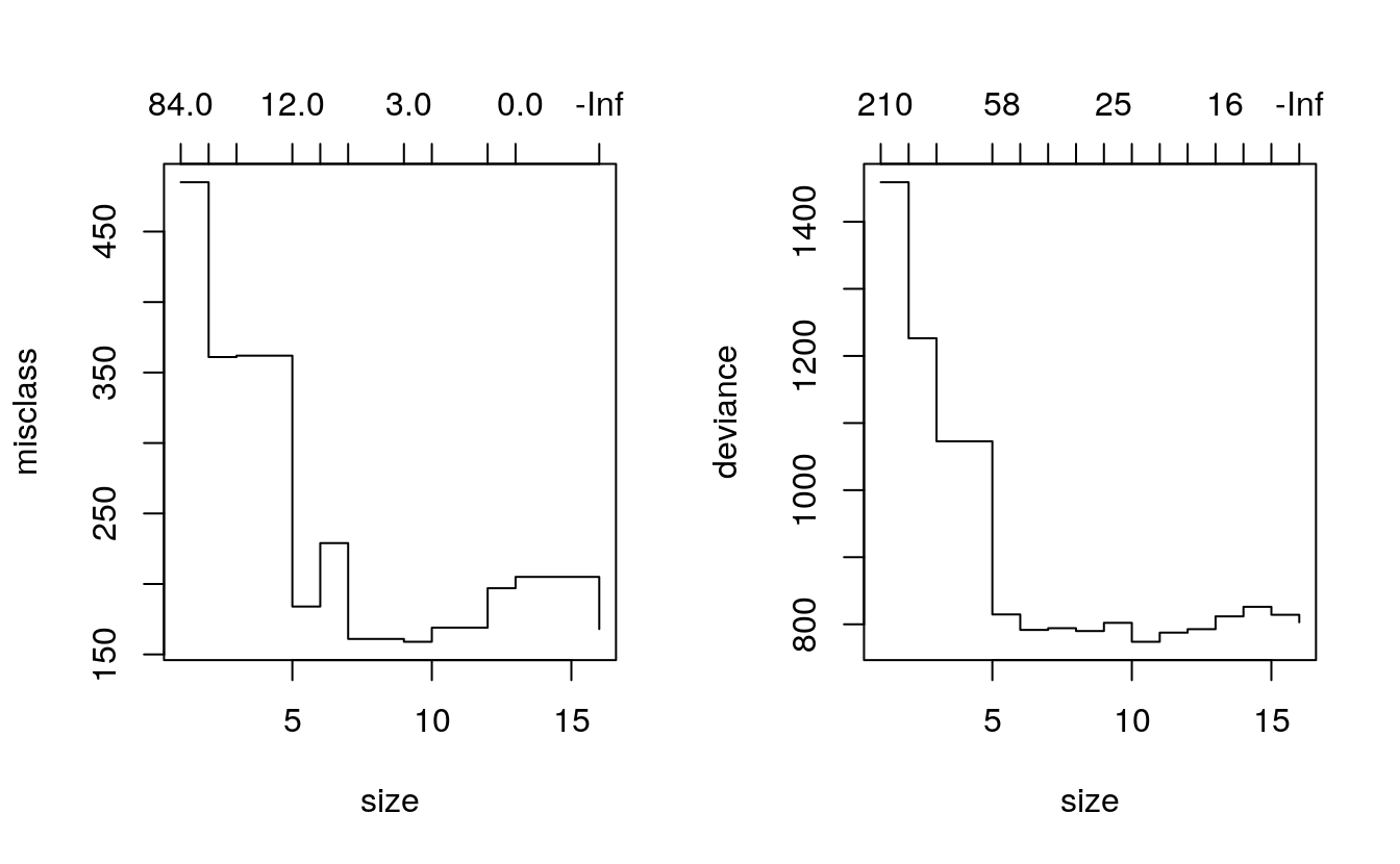
fitM.cv <- cv.tree(fit, K=346, FUN = prune.misclass)
fitP.cv <- cv.tree(fit, K=346, FUN = prune.tree)
The results are plotted out side by side in Figure 1.2. The jagged lines shows where the minimum deviance / misclassification occurred with the cross-validated tree. Since the cross validated misclassification and deviance both reach their minimum close to the number of branches in the original fitted tree there is little to be gained from pruning this tree
25.5 Make predictions
We use the validation data set and the fitted decision tree to predict vehicle classes; then we display the confusion matrix and calculate the error rate of the fitted tree. Overall, the model has an error rate of 32%.
testLabels <- Vehicle$Class[-train]
testLabels
#>   [1] van  bus  bus  van  van  bus  bus  saab opel bus  van  saab van  saab saab
#>  [16] van  saab opel van  saab saab saab bus  bus  saab opel bus  opel bus  opel
#>  [31] van  opel opel saab saab bus  bus  bus  van  van  saab opel bus  opel van
#>  [46] opel saab bus  van  bus  opel van  saab bus  opel bus  opel opel van  bus
#>  [61] van  saab opel bus  van  saab opel opel saab saab saab opel bus  van  bus
#>  [76] opel bus  saab bus  bus  bus  opel opel van  saab bus  bus  bus  van  saab
#>  [91] opel van  van  bus  bus  opel bus  opel saab opel bus  opel bus  saab van
#> [106] van  saab saab bus  van  opel van  saab opel saab saab van  van  van  van
#> [121] bus  bus  opel bus  bus  van  saab bus  opel bus  bus  bus  bus  opel van
#> [136] saab saab bus  opel van  bus  saab bus  van  bus  opel van  saab opel saab
#> [151] opel van  saab van  saab opel bus  van  bus  saab saab opel opel bus  bus
#> [166] opel van  van  bus  van  van  saab bus  saab opel saab opel bus  bus  bus
#> [181] saab bus  opel opel saab saab saab van  van  opel opel van  van  opel bus
#> [196] saab bus  van  opel opel bus  bus  bus  opel saab opel van  bus  opel opel
#> [211] saab opel bus  opel opel opel van  opel van  saab saab van  saab saab saab
#> [226] saab van  van  van  saab bus  van  van  bus  saab opel saab saab opel saab
#> [241] saab saab saab van  saab opel bus  saab bus  opel opel opel saab bus  van
#> [256] opel saab opel bus  bus  saab van  opel bus  saab van  opel saab saab saab
#> [271] saab van  opel bus  bus  bus  opel saab saab saab van  saab bus  opel saab
#> [286] van  opel bus  saab saab opel opel van  saab bus  opel bus  van  van  opel
#> [301] bus  bus  saab bus  van  saab bus  van  saab van  opel bus  bus  opel saab
#> [316] opel bus  bus  saab van  saab saab bus  opel opel opel bus  saab bus  van
#> [331] bus  van  saab opel saab van  opel opel van  bus  saab saab van  saab opel
#> [346] saab
#> Levels: bus opel saab van
# Confusion Matrix
pred <- predict(fit, newdata = testset)
# find column whih has the maximum of all rows
pred.class <- colnames(pred)[max.col(pred, ties.method = c("random"))]
cm <- table(testLabels, pred.class,
      dnn = c("Observed Class", "Predicted Class"))
cm
#>               Predicted Class
#> Observed Class bus opel saab van
#>           bus   85    1    1   5
#>           opel   3   70   10   2
#>           saab   7   67   14   7
#>           van    1    4    5  64
# pred <- predict(fit, newdata = Vehicle[-train,])
# pred.class <- colnames(pred)[max.col(pred, ties.method = c("random"))]
# table(Vehicle$Class[-train], pred.class,
#       dnn = c("Observed Class", "Predicted Class"))
# error_rate = (1 - sum(pred.class == Vehicle$Class[-train])/346)
# round(error_rate,3)