33 Comparison of six Linear Regression algorithms
- Datasets:
Boston - Algorithms:
- LM, GKM, GLMNET, SVM, CART, KNN
- Objective: Comparison of various algorithms
33.1 Introduction
These are the algorithms used:
- LM
- GLM
- GLMNET
- SVM
- CART
- KNN
# load packages
library(mlbench)
library(caret)
#> Loading required package: lattice
#> Loading required package: ggplot2
library(corrplot)
#> corrplot 0.84 loaded

# attach the BostonHousing dataset
data(BostonHousing)
dplyr::glimpse(BostonHousing)
#> Rows: 506
#> Columns: 14
#> $ crim    <dbl> 0.00632, 0.02731, 0.02729, 0.03237, 0.06905, 0.02985, 0.08829…
#> $ zn      <dbl> 18.0, 0.0, 0.0, 0.0, 0.0, 0.0, 12.5, 12.5, 12.5, 12.5, 12.5, …
#> $ indus   <dbl> 2.31, 7.07, 7.07, 2.18, 2.18, 2.18, 7.87, 7.87, 7.87, 7.87, 7…
#> $ chas    <fct> 0, 0, 0, 0, 0, 0, 0, 0, 0, 0, 0, 0, 0, 0, 0, 0, 0, 0, 0, 0, 0…
#> $ nox     <dbl> 0.538, 0.469, 0.469, 0.458, 0.458, 0.458, 0.524, 0.524, 0.524…
#> $ rm      <dbl> 6.58, 6.42, 7.18, 7.00, 7.15, 6.43, 6.01, 6.17, 5.63, 6.00, 6…
#> $ age     <dbl> 65.2, 78.9, 61.1, 45.8, 54.2, 58.7, 66.6, 96.1, 100.0, 85.9, …
#> $ dis     <dbl> 4.09, 4.97, 4.97, 6.06, 6.06, 6.06, 5.56, 5.95, 6.08, 6.59, 6…
#> $ rad     <dbl> 1, 2, 2, 3, 3, 3, 5, 5, 5, 5, 5, 5, 5, 4, 4, 4, 4, 4, 4, 4, 4…
#> $ tax     <dbl> 296, 242, 242, 222, 222, 222, 311, 311, 311, 311, 311, 311, 3…
#> $ ptratio <dbl> 15.3, 17.8, 17.8, 18.7, 18.7, 18.7, 15.2, 15.2, 15.2, 15.2, 1…
#> $ b       <dbl> 397, 397, 393, 395, 397, 394, 396, 397, 387, 387, 393, 397, 3…
#> $ lstat   <dbl> 4.98, 9.14, 4.03, 2.94, 5.33, 5.21, 12.43, 19.15, 29.93, 17.1…
#> $ medv    <dbl> 24.0, 21.6, 34.7, 33.4, 36.2, 28.7, 22.9, 27.1, 16.5, 18.9, 1…
tibble::as_tibble(BostonHousing)
#> # A tibble: 506 x 14
#>      crim    zn indus chas    nox    rm   age   dis   rad   tax ptratio     b
#>     <dbl> <dbl> <dbl> <fct> <dbl> <dbl> <dbl> <dbl> <dbl> <dbl>   <dbl> <dbl>
#> 1 0.00632    18  2.31 0     0.538  6.58  65.2  4.09     1   296    15.3  397.
#> 2 0.0273      0  7.07 0     0.469  6.42  78.9  4.97     2   242    17.8  397.
#> 3 0.0273      0  7.07 0     0.469  7.18  61.1  4.97     2   242    17.8  393.
#> 4 0.0324      0  2.18 0     0.458  7.00  45.8  6.06     3   222    18.7  395.
#> 5 0.0690      0  2.18 0     0.458  7.15  54.2  6.06     3   222    18.7  397.
#> 6 0.0298      0  2.18 0     0.458  6.43  58.7  6.06     3   222    18.7  394.
#> # … with 500 more rows, and 2 more variables: lstat <dbl>, medv <dbl>
33.2 Workflow
- Load dataset
- Create train and test datasets, 80/20
- Inspect dataset:
- Dimension
- classes
skimr
- Analyze features
- correlation
- Visualize features
- histograms
- density plots
- pairwise
- correlogram
- Train as-is
- Set the train control to
- 10 cross-validations
- 3 repetitions
- Metric: RMSE
- Train the models
- Compare accuracy of models
- Visual comparison
- dot plot
- Train with Feature selection
- Feature selection
findCorrelation- generate new dataset
- Train models again
- Compare RMSE again
- Visual comparison
- dot plot
- dot plot
- Train with dataset transformation
- data transformatiom
- Center
- Scale
- BoxCox
- Train models
- Compare RMSE
- Visual comparison
- dot plot
- Tune the best model
- Set the train control to
- 10 cross-validations
- 3 repetitions
- Metric: RMSE
- Train the models
- Radial SVM
- Sigma vector
- .C
- BoxCox 9, Ensembling
- Select the algorithms
- Random Forest
- Stochastic Gradient Boosting
- Cubist
- Numeric comparison
- resample
- summary
- Visual comparison
- dot plot
- Tune the best model: Cubist
- Set the train control to
- 10 cross-validations
- 3 repetitions
- Metric: RMSE
- Train the models
- Cubist
.committees.neighbors- BoxCox
- Evaluate the tuning parameters
- Numeric comparison
- print tuned model
- Visual comparison
- scatter plot
- Numeric comparison
- Finalize the model
- Back transformation
- Summary
- Apply model to validation set
- Transform the dataset
- Make prediction
- Calculate the RMSE
33.3 Preparing the data
# Split out validation dataset
# create a list of 80% of the rows in the original dataset we can use for training
set.seed(7)
validationIndex <- createDataPartition(BostonHousing$medv,
                                       p=0.80, list=FALSE)

# select 20% of the data for validation
validation <- BostonHousing[-validationIndex,]

# use the remaining 80% of data to training and testing the models
dataset <- BostonHousing[validationIndex,]
# list types for each attribute
sapply(dataset, class)
#>      crim        zn     indus      chas       nox        rm       age       dis
#> "numeric" "numeric" "numeric"  "factor" "numeric" "numeric" "numeric" "numeric"
#>       rad       tax   ptratio         b     lstat      medv
#> "numeric" "numeric" "numeric" "numeric" "numeric" "numeric"
# take a peek at the first 20 rows of the data
head(dataset, n=20)
#>       crim   zn indus chas   nox   rm   age  dis rad tax ptratio   b lstat medv
#> 1  0.00632 18.0  2.31    0 0.538 6.58  65.2 4.09   1 296    15.3 397  4.98 24.0
#> 2  0.02731  0.0  7.07    0 0.469 6.42  78.9 4.97   2 242    17.8 397  9.14 21.6
#> 3  0.02729  0.0  7.07    0 0.469 7.18  61.1 4.97   2 242    17.8 393  4.03 34.7
#> 4  0.03237  0.0  2.18    0 0.458 7.00  45.8 6.06   3 222    18.7 395  2.94 33.4
#> 5  0.06905  0.0  2.18    0 0.458 7.15  54.2 6.06   3 222    18.7 397  5.33 36.2
#> 6  0.02985  0.0  2.18    0 0.458 6.43  58.7 6.06   3 222    18.7 394  5.21 28.7
#> 7  0.08829 12.5  7.87    0 0.524 6.01  66.6 5.56   5 311    15.2 396 12.43 22.9
#> 10 0.17004 12.5  7.87    0 0.524 6.00  85.9 6.59   5 311    15.2 387 17.10 18.9
#> 11 0.22489 12.5  7.87    0 0.524 6.38  94.3 6.35   5 311    15.2 393 20.45 15.0
#> 12 0.11747 12.5  7.87    0 0.524 6.01  82.9 6.23   5 311    15.2 397 13.27 18.9
#> 13 0.09378 12.5  7.87    0 0.524 5.89  39.0 5.45   5 311    15.2 390 15.71 21.7
#> 14 0.62976  0.0  8.14    0 0.538 5.95  61.8 4.71   4 307    21.0 397  8.26 20.4
#> 15 0.63796  0.0  8.14    0 0.538 6.10  84.5 4.46   4 307    21.0 380 10.26 18.2
#> 17 1.05393  0.0  8.14    0 0.538 5.93  29.3 4.50   4 307    21.0 387  6.58 23.1
#> 20 0.72580  0.0  8.14    0 0.538 5.73  69.5 3.80   4 307    21.0 391 11.28 18.2
#> 21 1.25179  0.0  8.14    0 0.538 5.57  98.1 3.80   4 307    21.0 377 21.02 13.6
#> 22 0.85204  0.0  8.14    0 0.538 5.96  89.2 4.01   4 307    21.0 393 13.83 19.6
#> 23 1.23247  0.0  8.14    0 0.538 6.14  91.7 3.98   4 307    21.0 397 18.72 15.2
#> 24 0.98843  0.0  8.14    0 0.538 5.81 100.0 4.10   4 307    21.0 395 19.88 14.5
#> 25 0.75026  0.0  8.14    0 0.538 5.92  94.1 4.40   4 307    21.0 394 16.30 15.6
library(skimr)
print(skim_with(numeric = list(hist = NULL)))
#> Creating new skimming functions for the following classes: hist.
#> They did not have recognized defaults. Call get_default_skimmers() for more information.
#> function(data, ...) {
#>     data_name <- rlang::expr_label(substitute(data))
#>     if (!inherits(data, "data.frame")) {
#>       data <- as.data.frame(data)
#>     }
#>     stopifnot(inherits(data, "data.frame"))
#>
#>     .vars <- rlang::quos(...)
#>     cols <- names(data)
#>     if (length(.vars) == 0) {
#>       selected <- cols
#>     } else {
#>       selected <- tidyselect::vars_select(cols, !!!.vars)
#>     }
#>
#>     grps <- dplyr::groups(data)
#>     if (length(grps) > 0) {
#>       group_variables <- selected %in% as.character(grps)
#>       selected <- selected[!group_variables]
#>     } else {
#>       attr(data, "groups") <- list()
#>     }
#>
#>
#>     skimmers <- purrr::map(
#>       selected, get_final_skimmers, data, local_skimmers, append
#>     )
#>     types <- purrr::map_chr(skimmers, "skim_type")
#>     unique_skimmers <- reduce_skimmers(skimmers, types)
#>     combined_skimmers <- purrr::map(unique_skimmers, join_with_base, base)
#>     ready_to_skim <- tibble::tibble(
#>       skim_type = unique(types),
#>       skimmers = purrr::map(combined_skimmers, mangle_names, names(base$funs)),
#>       skim_variable = split(selected, types)[unique(types)]
#>     )
#>     grouped <- dplyr::group_by(ready_to_skim, .data$skim_type)
#>     nested <- dplyr::summarize(
#>       grouped,
#>       skimmed = purrr::map2(
#>         .data$skimmers, .data$skim_variable, skim_by_type, data
#>       )
#>     )
#>     structure(
#>       tidyr::unnest(nested, .data$skimmed),
#>       class = c("skim_df", "tbl_df", "tbl", "data.frame"),
#>       data_rows = nrow(data),
#>       data_cols = ncol(data),
#>       df_name = data_name,
#>       groups = dplyr::groups(data),
#>       base_skimmers = names(base$funs),
#>       skimmers_used = get_skimmers_used(unique_skimmers)
#>     )
#>   }
#> <bytecode: 0x5618f38e5c70>
#> <environment: 0x5618f38ac0c0>
print(skim(dataset))
#> ── Data Summary ────────────────────────
#>                            Values
#> Name                       dataset
#> Number of rows             407
#> Number of columns          14
#> _______________________
#> Column type frequency:
#>   factor                   1
#>   numeric                  13
#> ________________________
#> Group variables            None
#>
#> ── Variable type: factor ───────────────────────────────────────────────────────
#>   skim_variable n_missing complete_rate ordered n_unique top_counts
#> 1 chas                  0             1 FALSE          2 0: 378, 1: 29
#>
#> ── Variable type: numeric ──────────────────────────────────────────────────────
#>    skim_variable n_missing complete_rate    mean      sd        p0      p25
#>  1 crim                  0             1   3.64    8.80    0.00632   0.0796
#>  2 zn                    0             1  11.9    24.2     0         0
#>  3 indus                 0             1  11.0     6.87    0.74      4.93
#>  4 nox                   0             1   0.555   0.117   0.385     0.448
#>  5 rm                    0             1   6.29    0.704   3.56      5.89
#>  6 age                   0             1  68.4    28.2     6.2      42.7
#>  7 dis                   0             1   3.82    2.12    1.13      2.11
#>  8 rad                   0             1   9.59    8.77    1         4
#>  9 tax                   0             1 409.    169.    187       280.
#> 10 ptratio               0             1  18.4     2.18   12.6      17
#> 11 b                     0             1 357.     89.7     0.32    374.
#> 12 lstat                 0             1  12.6     7.03    1.92      7.06
#> 13 medv                  0             1  22.5     8.96    5        17.0
#>        p50     p75    p100 hist
#>  1   0.268   3.69   89.0   ▇▁▁▁▁
#>  2   0      15     100     ▇▁▁▁▁
#>  3   8.56   18.1    27.7   ▇▆▁▇▁
#>  4   0.538   0.631   0.871 ▇▇▆▃▁
#>  5   6.21    6.62    8.78  ▁▁▇▂▁
#>  6  77.3    94.2   100     ▂▃▂▂▇
#>  7   3.15    5.21   12.1   ▇▅▂▁▁
#>  8   5      24      24     ▇▂▁▁▃
#>  9 334     666     711     ▇▇▃▁▇
#> 10  19      20.2    22     ▁▃▅▅▇
#> 11 391.    396.    397.    ▁▁▁▁▇
#> 12  11.3    16.5    38.0   ▇▇▃▂▁
#> 13  21.2    25      50     ▂▇▃▁▁
dataset[,4] <- as.numeric(as.character(dataset[,4]))
print(skim(dataset))
#> ── Data Summary ────────────────────────
#>                            Values
#> Name                       dataset
#> Number of rows             407
#> Number of columns          14
#> _______________________
#> Column type frequency:
#>   numeric                  14
#> ________________________
#> Group variables            None
#>
#> ── Variable type: numeric ──────────────────────────────────────────────────────
#>    skim_variable n_missing complete_rate     mean      sd        p0      p25
#>  1 crim                  0             1   3.64     8.80    0.00632   0.0796
#>  2 zn                    0             1  11.9     24.2     0         0
#>  3 indus                 0             1  11.0      6.87    0.74      4.93
#>  4 chas                  0             1   0.0713   0.258   0         0
#>  5 nox                   0             1   0.555    0.117   0.385     0.448
#>  6 rm                    0             1   6.29     0.704   3.56      5.89
#>  7 age                   0             1  68.4     28.2     6.2      42.7
#>  8 dis                   0             1   3.82     2.12    1.13      2.11
#>  9 rad                   0             1   9.59     8.77    1         4
#> 10 tax                   0             1 409.     169.    187       280.
#> 11 ptratio               0             1  18.4      2.18   12.6      17
#> 12 b                     0             1 357.      89.7     0.32    374.
#> 13 lstat                 0             1  12.6      7.03    1.92      7.06
#> 14 medv                  0             1  22.5      8.96    5        17.0
#>        p50     p75    p100 hist
#>  1   0.268   3.69   89.0   ▇▁▁▁▁
#>  2   0      15     100     ▇▁▁▁▁
#>  3   8.56   18.1    27.7   ▇▆▁▇▁
#>  4   0       0       1     ▇▁▁▁▁
#>  5   0.538   0.631   0.871 ▇▇▆▃▁
#>  6   6.21    6.62    8.78  ▁▁▇▂▁
#>  7  77.3    94.2   100     ▂▃▂▂▇
#>  8   3.15    5.21   12.1   ▇▅▂▁▁
#>  9   5      24      24     ▇▂▁▁▃
#> 10 334     666     711     ▇▇▃▁▇
#> 11  19      20.2    22     ▁▃▅▅▇
#> 12 391.    396.    397.    ▁▁▁▁▇
#> 13  11.3    16.5    38.0   ▇▇▃▂▁
#> 14  21.2    25      50     ▂▇▃▁▁
no more factors or character variables
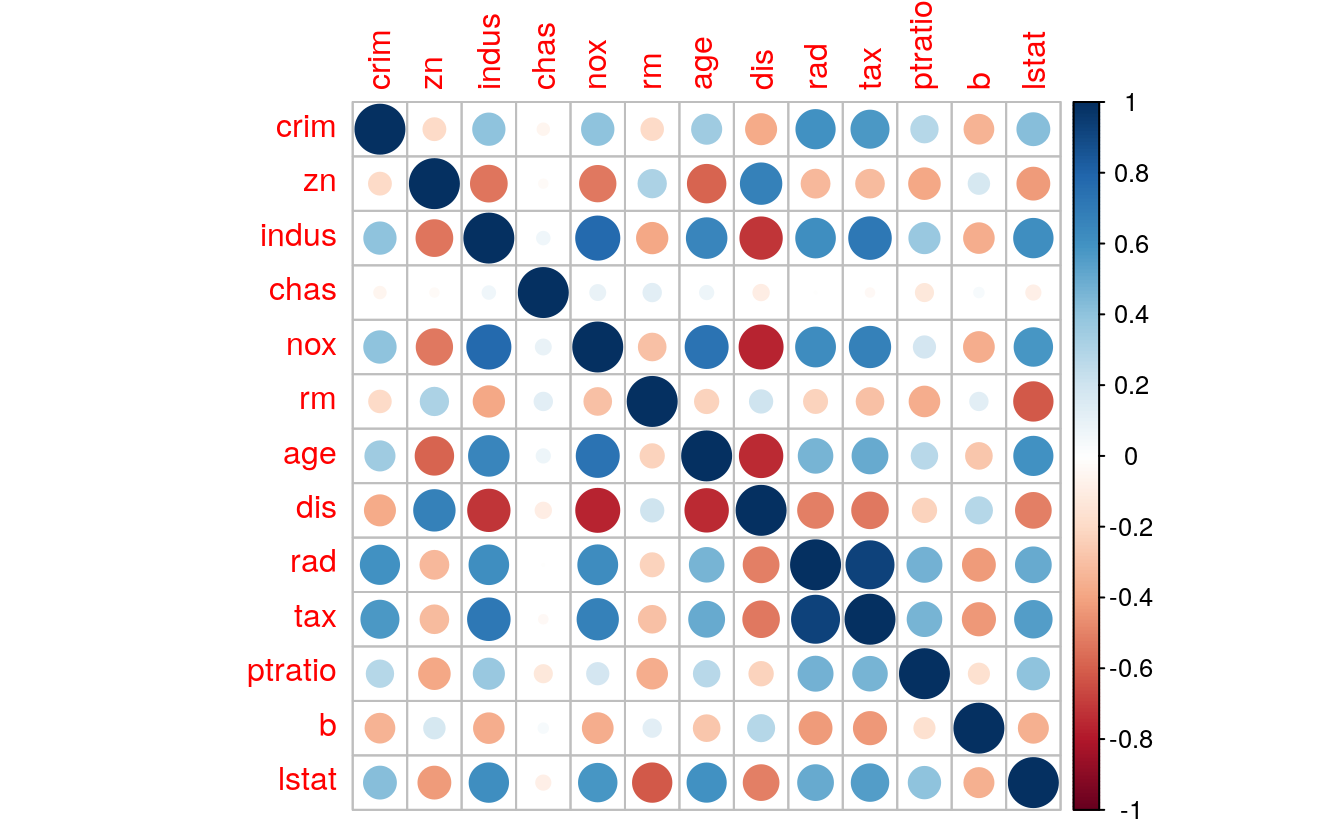
33.3.1 Variables correlation
# find correlation between variables
cor(dataset[,1:13])
#>            crim      zn   indus     chas     nox     rm     age    dis      rad
#> crim     1.0000 -0.1996  0.4076 -0.05507  0.4099 -0.194  0.3524 -0.376  0.60834
#> zn      -0.1996  1.0000 -0.5314 -0.02987 -0.5202  0.311 -0.5845  0.680 -0.32273
#> indus    0.4076 -0.5314  1.0000  0.06583  0.7733 -0.383  0.6512 -0.711  0.61998
#> chas    -0.0551 -0.0299  0.0658  1.00000  0.0934  0.127  0.0735 -0.099 -0.00245
#> nox      0.4099 -0.5202  0.7733  0.09340  1.0000 -0.296  0.7338 -0.769  0.62760
#> rm      -0.1940  0.3111 -0.3826  0.12677 -0.2961  1.000 -0.2262  0.207 -0.22126
#> age      0.3524 -0.5845  0.6512  0.07350  0.7338 -0.226  1.0000 -0.749  0.46896
#> dis     -0.3756  0.6799 -0.7113 -0.09905 -0.7693  0.207 -0.7492  1.000 -0.50372
#> rad      0.6083 -0.3227  0.6200 -0.00245  0.6276 -0.221  0.4690 -0.504  1.00000
#> tax      0.5711 -0.3184  0.7185 -0.03064  0.6758 -0.295  0.5058 -0.526  0.92005
#> ptratio  0.2897 -0.3888  0.3782 -0.12283  0.1888 -0.365  0.2709 -0.228  0.47971
#> b       -0.3442  0.1747 -0.3644  0.03782 -0.3684  0.126 -0.2742  0.284 -0.42314
#> lstat    0.4229 -0.4219  0.6136 -0.08430  0.5839 -0.612  0.6066 -0.501  0.50251
#>             tax ptratio       b   lstat
#> crim     0.5711   0.290 -0.3442  0.4229
#> zn      -0.3184  -0.389  0.1747 -0.4219
#> indus    0.7185   0.378 -0.3644  0.6136
#> chas    -0.0306  -0.123  0.0378 -0.0843
#> nox      0.6758   0.189 -0.3684  0.5839
#> rm      -0.2953  -0.365  0.1260 -0.6120
#> age      0.5058   0.271 -0.2742  0.6066
#> dis     -0.5264  -0.228  0.2843 -0.5013
#> rad      0.9201   0.480 -0.4231  0.5025
#> tax      1.0000   0.469 -0.4303  0.5538
#> ptratio  0.4691   1.000 -0.1700  0.4093
#> b       -0.4303  -0.170  1.0000 -0.3509
#> lstat    0.5538   0.409 -0.3509  1.0000
library(dplyr)
#>
#> Attaching package: 'dplyr'
#> The following objects are masked from 'package:stats':
#>
#>     filter, lag
#> The following objects are masked from 'package:base':
#>
#>     intersect, setdiff, setequal, union

m <- cor(dataset[,1:13])
diag(m) <- 0
# select variables with correlation 0.7 and above
threshold <- 0.7
ok <- apply(abs(m) >= threshold, 1, any)
m[ok, ok]
#>        indus    nox    age    dis    rad    tax
#> indus  0.000  0.773  0.651 -0.711  0.620  0.719
#> nox    0.773  0.000  0.734 -0.769  0.628  0.676
#> age    0.651  0.734  0.000 -0.749  0.469  0.506
#> dis   -0.711 -0.769 -0.749  0.000 -0.504 -0.526
#> rad    0.620  0.628  0.469 -0.504  0.000  0.920
#> tax    0.719  0.676  0.506 -0.526  0.920  0.000
# values of correlation >= 0.7
ind <- sapply(1:13, function(x) abs(m[, x]) > 0.7)
m[ind]
#>  [1]  0.773 -0.711  0.719  0.773  0.734 -0.769  0.734 -0.749 -0.711 -0.769
#> [11] -0.749  0.920  0.719  0.920
# defining a index for selecting if the condition is met
cind <- apply(m, 2, function(x) any(abs(x) > 0.7))
cm <- m[, cind] # since col6 only has values less than 0.5 it is not taken
cm
#>           indus     nox     age    dis      rad     tax
#> crim     0.4076  0.4099  0.3524 -0.376  0.60834  0.5711
#> zn      -0.5314 -0.5202 -0.5845  0.680 -0.32273 -0.3184
#> indus    0.0000  0.7733  0.6512 -0.711  0.61998  0.7185
#> chas     0.0658  0.0934  0.0735 -0.099 -0.00245 -0.0306
#> nox      0.7733  0.0000  0.7338 -0.769  0.62760  0.6758
#> rm      -0.3826 -0.2961 -0.2262  0.207 -0.22126 -0.2953
#> age      0.6512  0.7338  0.0000 -0.749  0.46896  0.5058
#> dis     -0.7113 -0.7693 -0.7492  0.000 -0.50372 -0.5264
#> rad      0.6200  0.6276  0.4690 -0.504  0.00000  0.9201
#> tax      0.7185  0.6758  0.5058 -0.526  0.92005  0.0000
#> ptratio  0.3782  0.1888  0.2709 -0.228  0.47971  0.4691
#> b       -0.3644 -0.3684 -0.2742  0.284 -0.42314 -0.4303
#> lstat    0.6136  0.5839  0.6066 -0.501  0.50251  0.5538
rind <- apply(cm, 1, function(x) any(abs(x) > 0.7))
rm <- cm[rind, ]
rm
#> indus nox age dis rad tax
#> indus 0.000 0.773 0.651 -0.711 0.620 0.719
#> nox 0.773 0.000 0.734 -0.769 0.628 0.676
#> age 0.651 0.734 0.000 -0.749 0.469 0.506
#> dis -0.711 -0.769 -0.749 0.000 -0.504 -0.526
#> rad 0.620 0.628 0.469 -0.504 0.000 0.920
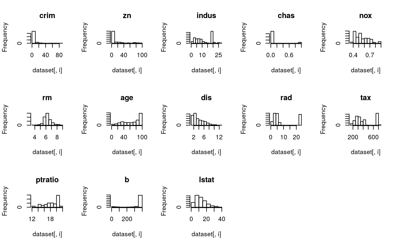
#> tax 0.719 0.676 0.506 -0.526 0.920 0.00033.3.2 A look at the variables
# histograms for each attribute
par(mfrow=c(3,5))
for(i in 1:13) {
    hist(dataset[,i], main=names(dataset)[i])
}
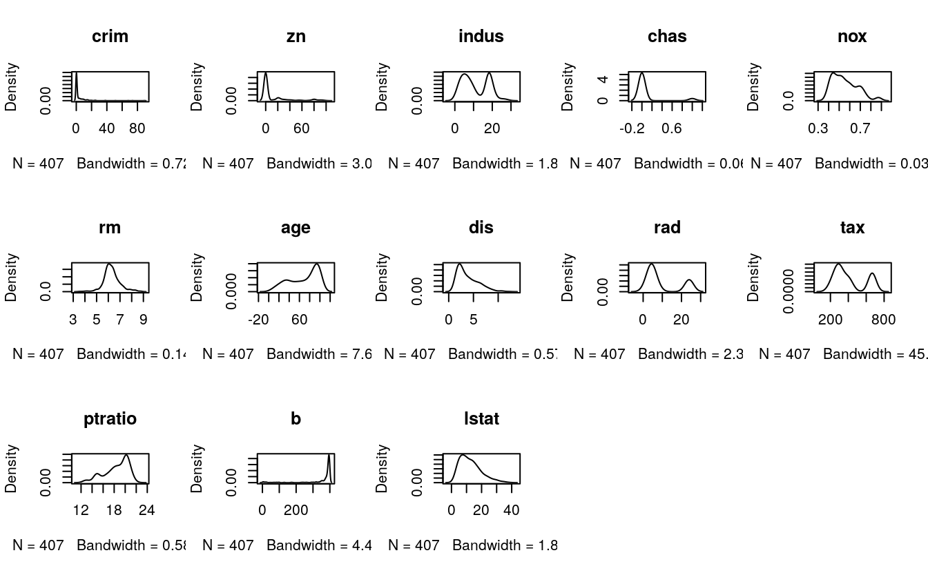
# density plot for each attribute
par(mfrow=c(3,5))
for(i in 1:13) {
plot(density(dataset[,i]), main=names(dataset)[i])
}
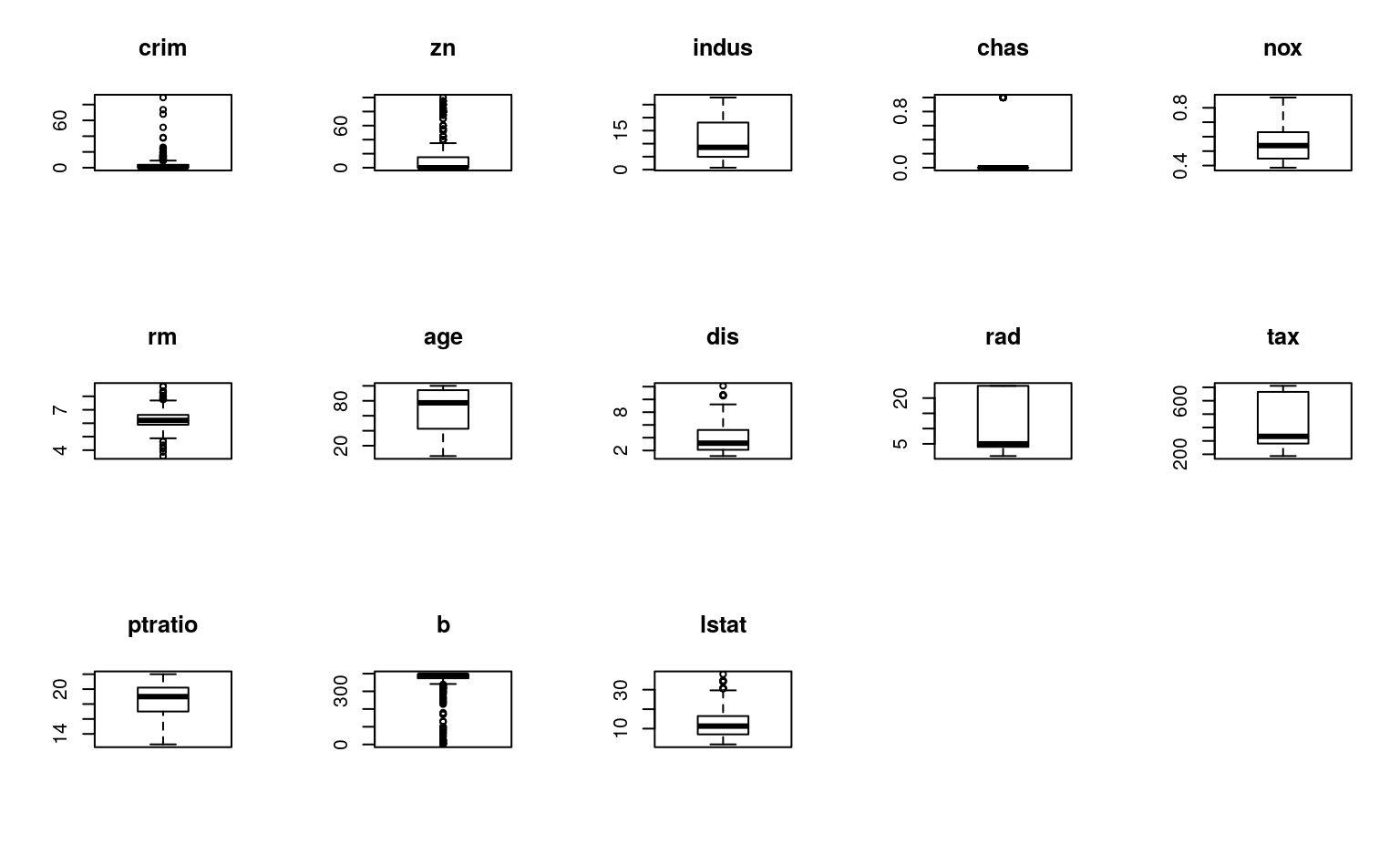
# boxplots for each attribute
par(mfrow=c(3,5))
for(i in 1:13) {
boxplot(dataset[,i], main=names(dataset)[i])
}
# scatter plot matrix
pairs(dataset[,1:13])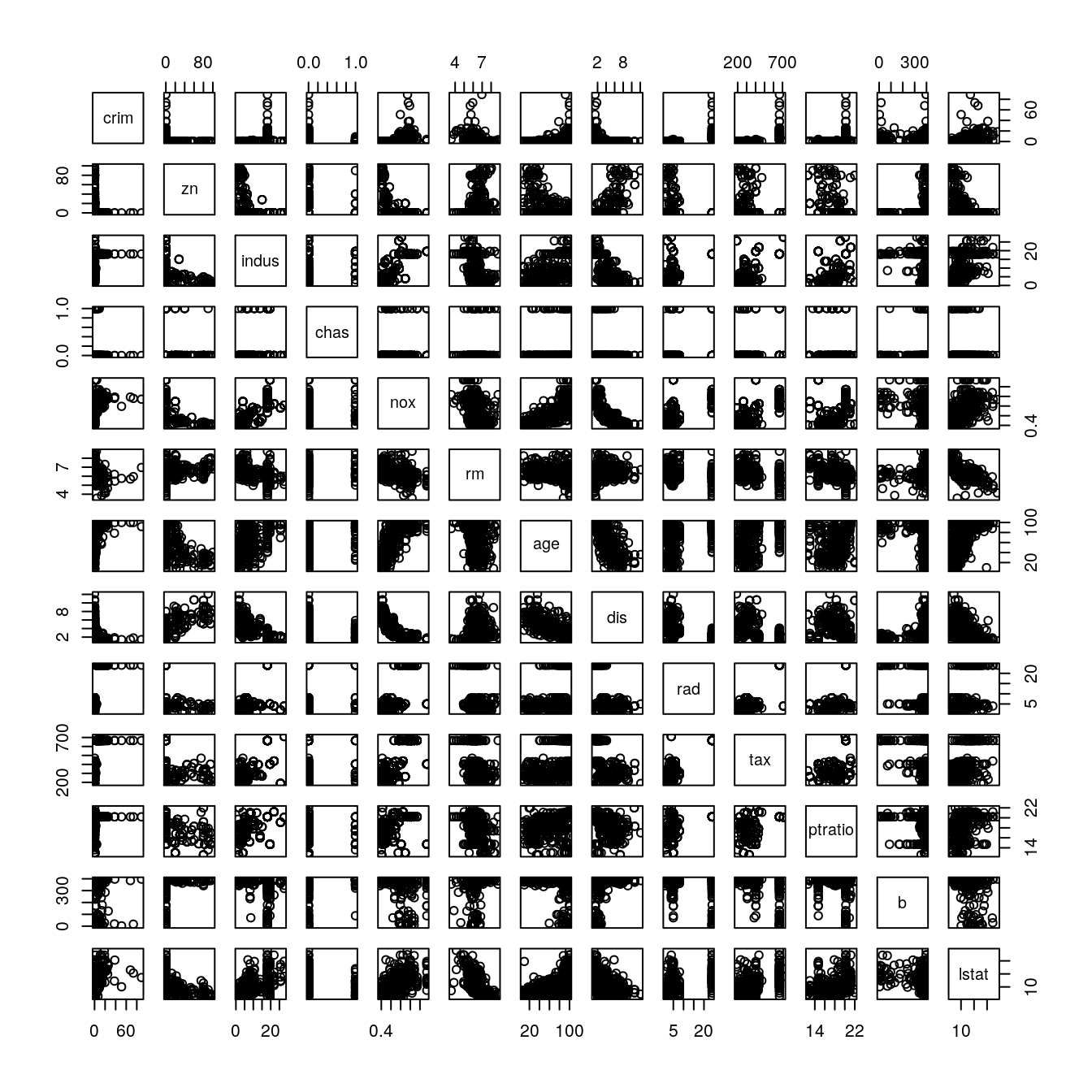
33.4 Evaluation of algorithms
# Run algorithms using 10-fold cross-validation
trainControl <- trainControl(method="repeatedcv", number=10, repeats=3)
metric <- "RMSE"
# LM
set.seed(7)
fit.lm <- train(medv~., data=dataset, method="lm",
                metric=metric, preProc=c("center", "scale"),
                trControl=trainControl)
# GLM
set.seed(7)
fit.glm <- train(medv~., data=dataset, method="glm",
                 metric=metric, preProc=c("center", "scale"),
                 trControl=trainControl)
# GLMNET
set.seed(7)
fit.glmnet <- train(medv~., data=dataset, method="glmnet",
                    metric=metric,
                    preProc=c("center", "scale"),
                    trControl=trainControl)
# SVM
set.seed(7)
fit.svm <- train(medv~., data=dataset, method="svmRadial",
                 metric=metric,
                 preProc=c("center", "scale"),
                 trControl=trainControl)
# CART
set.seed(7)
grid <- expand.grid(.cp=c(0, 0.05, 0.1))
fit.cart <- train(medv~., data=dataset, method="rpart",
                  metric=metric, tuneGrid=grid,
                  preProc=c("center", "scale"),
                  trControl=trainControl)
# KNN
set.seed(7)
fit.knn <- train(medv~., data=dataset, method="knn",
                 metric=metric, preProc=c("center", "scale"),
                 trControl=trainControl)
# Compare algorithms
results <- resamples(list(LM     = fit.lm,
                          GLM    = fit.glm,
                          GLMNET = fit.glmnet,
                          SVM    = fit.svm,
                          CART   = fit.cart,
                          KNN    = fit.knn))
summary(results)
#>
#> Call:
#> summary.resamples(object = results)
#>
#> Models: LM, GLM, GLMNET, SVM, CART, KNN
#> Number of resamples: 30
#>
#> MAE
#>        Min. 1st Qu. Median Mean 3rd Qu. Max. NA's
#> LM     2.30    2.90   3.37 3.32    3.70 4.64    0
#> GLM    2.30    2.90   3.37 3.32    3.70 4.64    0
#> GLMNET 2.30    2.88   3.34 3.30    3.70 4.63    0
#> SVM    1.42    1.99   2.52 2.39    2.65 3.35    0
#> CART   2.22    2.62   2.88 2.93    3.08 4.16    0
#> KNN    1.98    2.69   2.87 2.95    3.24 4.00    0
#>
#> RMSE
#>        Min. 1st Qu. Median Mean 3rd Qu. Max. NA's
#> LM     2.99    3.87   4.63 4.63    5.32 6.69    0
#> GLM    2.99    3.87   4.63 4.63    5.32 6.69    0
#> GLMNET 2.99    3.88   4.62 4.62    5.32 6.69    0
#> SVM    2.05    2.95   3.81 3.91    4.46 6.98    0
#> CART   2.77    3.38   4.00 4.20    4.60 7.09    0
#> KNN    2.65    3.74   4.42 4.48    5.06 6.98    0
#>
#> Rsquared
#>         Min. 1st Qu. Median  Mean 3rd Qu.  Max. NA's
#> LM     0.505   0.674  0.747 0.740   0.813 0.900    0
#> GLM    0.505   0.674  0.747 0.740   0.813 0.900    0
#> GLMNET 0.503   0.673  0.747 0.741   0.816 0.904    0
#> SVM    0.519   0.762  0.845 0.810   0.896 0.970    0
#> CART   0.514   0.737  0.816 0.778   0.842 0.899    0
#> KNN    0.519   0.748  0.804 0.770   0.829 0.931    0
dotplot(results)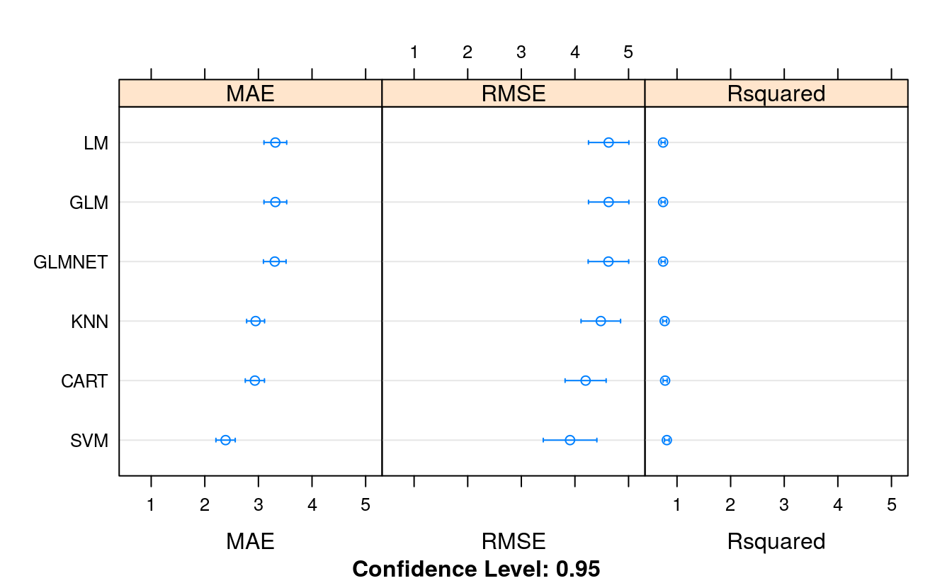
33.5 Feature selection
# remove correlated attributes
# find attributes that are highly correlated
set.seed(7)
cutoff <- 0.70
correlations <- cor(dataset[,1:13])
highlyCorrelated <- findCorrelation(correlations, cutoff=cutoff)

for (value in highlyCorrelated) {
    print(names(dataset)[value])
}
#> [1] "indus"
#> [1] "nox"
#> [1] "tax"
#> [1] "dis"

# create a new dataset without highly correlated features
datasetFeatures <- dataset[,-highlyCorrelated]
dim(datasetFeatures)
#> [1] 407  10
# Run algorithms using 10-fold cross-validation
trainControl <- trainControl(method="repeatedcv", number=10, repeats=3)
metric <- "RMSE"

# LM
set.seed(7)
fit.lm <- train(medv~., data=dataset, method="lm",
                metric=metric, preProc=c("center", "scale"),
                trControl=trainControl)
# GLM
set.seed(7)
fit.glm <- train(medv~., data=dataset, method="glm",
                 metric=metric, preProc=c("center", "scale"),
                 trControl=trainControl)
# GLMNET
set.seed(7)
fit.glmnet <- train(medv~., data=dataset, method="glmnet",
                    metric=metric,
                    preProc=c("center", "scale"),
                    trControl=trainControl)
# SVM
set.seed(7)
fit.svm <- train(medv~., data=dataset, method="svmRadial",
                 metric=metric,
                 preProc=c("center", "scale"),
                 trControl=trainControl)
# CART
set.seed(7)
grid <- expand.grid(.cp=c(0, 0.05, 0.1))
fit.cart <- train(medv~., data=dataset, method="rpart",
                  metric=metric, tuneGrid=grid,
                  preProc=c("center", "scale"),
                  trControl=trainControl)
# KNN
set.seed(7)
fit.knn <- train(medv~., data=dataset, method="knn",
                 metric=metric, preProc=c("center", "scale"),
                 trControl=trainControl)

# Compare algorithms
feature_results <- resamples(list(LM     = fit.lm,
                                  GLM    = fit.glm,
                                  GLMNET = fit.glmnet,
                                  SVM    = fit.svm,
                                  CART   = fit.cart,
                                  KNN    = fit.knn))
summary(feature_results)
#>
#> Call:
#> summary.resamples(object = feature_results)
#>
#> Models: LM, GLM, GLMNET, SVM, CART, KNN
#> Number of resamples: 30
#>
#> MAE
#>        Min. 1st Qu. Median Mean 3rd Qu. Max. NA's
#> LM     2.30    2.90   3.37 3.32    3.70 4.64    0
#> GLM    2.30    2.90   3.37 3.32    3.70 4.64    0
#> GLMNET 2.30    2.88   3.34 3.30    3.70 4.63    0
#> SVM    1.42    1.99   2.52 2.39    2.65 3.35    0
#> CART   2.22    2.62   2.88 2.93    3.08 4.16    0
#> KNN    1.98    2.69   2.87 2.95    3.24 4.00    0
#>
#> RMSE
#>        Min. 1st Qu. Median Mean 3rd Qu. Max. NA's
#> LM     2.99    3.87   4.63 4.63    5.32 6.69    0
#> GLM    2.99    3.87   4.63 4.63    5.32 6.69    0
#> GLMNET 2.99    3.88   4.62 4.62    5.32 6.69    0
#> SVM    2.05    2.95   3.81 3.91    4.46 6.98    0
#> CART   2.77    3.38   4.00 4.20    4.60 7.09    0
#> KNN    2.65    3.74   4.42 4.48    5.06 6.98    0
#>
#> Rsquared
#>         Min. 1st Qu. Median  Mean 3rd Qu.  Max. NA's
#> LM     0.505   0.674  0.747 0.740   0.813 0.900    0
#> GLM    0.505   0.674  0.747 0.740   0.813 0.900    0
#> GLMNET 0.503   0.673  0.747 0.741   0.816 0.904    0
#> SVM    0.519   0.762  0.845 0.810   0.896 0.970    0
#> CART   0.514   0.737  0.816 0.778   0.842 0.899    0
#> KNN    0.519   0.748  0.804 0.770   0.829 0.931    0
dotplot(feature_results)
Comparing the results, we can see that this has made the RMSE worse for the linear and the nonlinear algorithms. The correlated attributes we removed are contributing to the accuracy of the models.
33.6 Evaluate Algorithms: Box-Cox Transform
We know that some of the attributes have a skew and others perhaps have an
exponential distribution. One option would be to explore squaring and log
transforms respectively (you could try this!). Another approach would be to use a power transform and let it figure out the amount to correct each attribute. One example is the Box-Cox power transform. Let’s try using this transform to rescale the original data and evaluate the effect on the same 6 algorithms. We will also leave in the centering and scaling for the benefit of the instance-based methods.
# Run algorithms using 10-fold cross-validation
trainControl <- trainControl(method="repeatedcv", number=10, repeats=3)
metric <- "RMSE"

# lm
set.seed(7)
fit.lm <- train(medv~., data=dataset, method="lm", metric=metric,
                preProc=c("center", "scale", "BoxCox"),
                trControl=trainControl)
# GLM
set.seed(7)
fit.glm <- train(medv~., data=dataset, method="glm", metric=metric,
                 preProc=c("center", "scale", "BoxCox"),
                 trControl=trainControl)
# GLMNET
set.seed(7)
fit.glmnet <- train(medv~., data=dataset, method="glmnet", metric=metric,
                    preProc=c("center", "scale", "BoxCox"),
                    trControl=trainControl)
# SVM
set.seed(7)
fit.svm <- train(medv~., data=dataset, method="svmRadial", metric=metric,
                 preProc=c("center", "scale", "BoxCox"),
                 trControl=trainControl)
# CART
set.seed(7)
grid <- expand.grid(.cp=c(0, 0.05, 0.1))
fit.cart <- train(medv~., data=dataset, method="rpart", metric=metric,
                  tuneGrid=grid,
                  preProc=c("center", "scale", "BoxCox"),
                  trControl=trainControl)
# KNN
set.seed(7)
fit.knn <- train(medv~., data=dataset, method="knn", metric=metric,
                 preProc=c("center", "scale", "BoxCox"),
                 trControl=trainControl)

# Compare algorithms
transformResults <- resamples(list(LM     = fit.lm,
                                  GLM    = fit.glm,
                                  GLMNET = fit.glmnet,
                                  SVM    = fit.svm,
                                  CART   = fit.cart,
                                  KNN    = fit.knn))
summary(transformResults)
#>
#> Call:
#> summary.resamples(object = transformResults)
#>
#> Models: LM, GLM, GLMNET, SVM, CART, KNN
#> Number of resamples: 30
#>
#> MAE
#>        Min. 1st Qu. Median Mean 3rd Qu. Max. NA's
#> LM     2.10    2.80   3.21 3.18    3.45 4.44    0
#> GLM    2.10    2.80   3.21 3.18    3.45 4.44    0
#> GLMNET 2.11    2.80   3.21 3.17    3.45 4.43    0
#> SVM    1.30    1.95   2.25 2.26    2.48 3.19    0
#> CART   2.22    2.62   2.89 2.94    3.11 4.16    0
#> KNN    2.33    2.66   2.82 2.97    3.27 3.96    0
#>
#> RMSE
#>        Min. 1st Qu. Median Mean 3rd Qu. Max. NA's
#> LM     2.82    3.81   4.43 4.37    5.00 6.16    0
#> GLM    2.82    3.81   4.43 4.37    5.00 6.16    0
#> GLMNET 2.83    3.79   4.42 4.36    5.00 6.18    0
#> SVM    1.80    2.73   3.41 3.70    4.24 6.73    0
#> CART   2.77    3.38   4.00 4.23    4.83 7.09    0
#> KNN    3.01    3.73   4.37 4.52    5.02 7.30    0
#>
#> Rsquared
#>         Min. 1st Qu. Median  Mean 3rd Qu.  Max. NA's
#> LM     0.560   0.712  0.775 0.766   0.825 0.910    0
#> GLM    0.560   0.712  0.775 0.766   0.825 0.910    0
#> GLMNET 0.556   0.713  0.775 0.766   0.826 0.910    0
#> SVM    0.524   0.778  0.854 0.827   0.907 0.979    0
#> CART   0.514   0.727  0.816 0.774   0.843 0.899    0
#> KNN    0.492   0.723  0.792 0.762   0.842 0.937    0
dotplot(transformResults)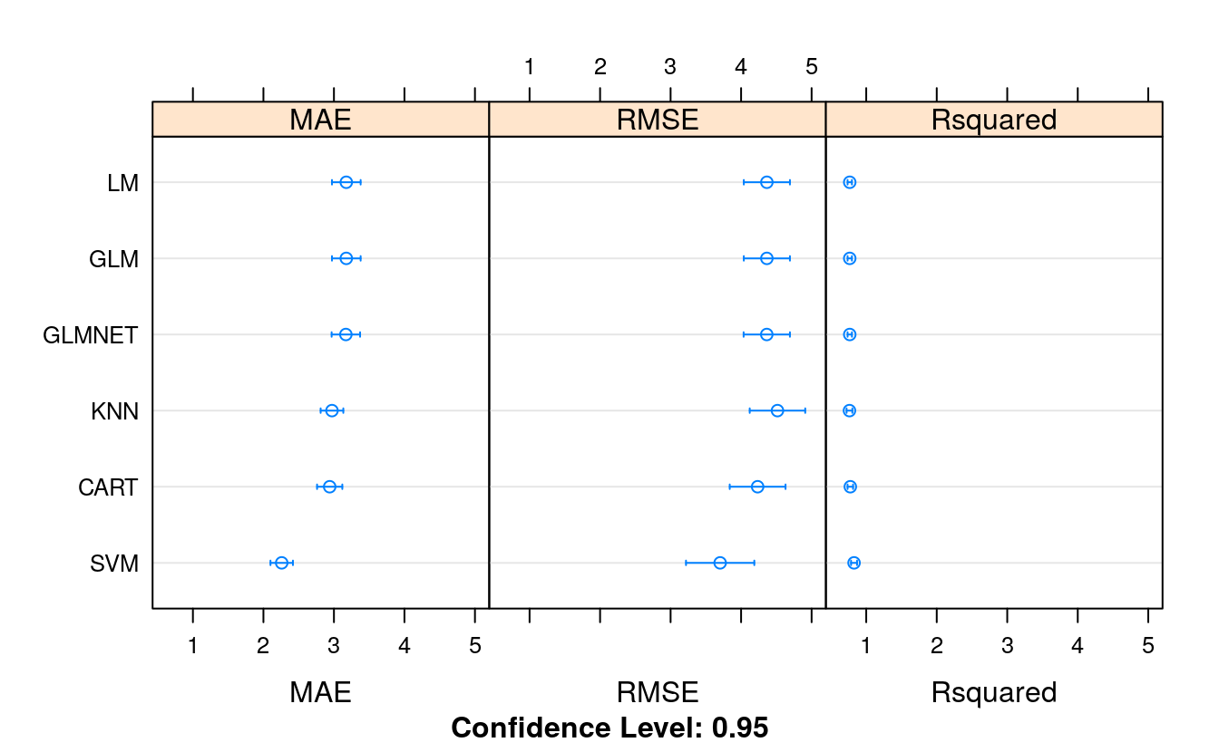
33.7 Tune SVM
print(fit.svm)
#> Support Vector Machines with Radial Basis Function Kernel
#>
#> 407 samples
#>  13 predictor
#>
#> Pre-processing: centered (13), scaled (13), Box-Cox transformation (11)
#> Resampling: Cross-Validated (10 fold, repeated 3 times)
#> Summary of sample sizes: 365, 366, 366, 367, 366, 366, ...
#> Resampling results across tuning parameters:
#>
#>   C     RMSE  Rsquared  MAE
#>   0.25  4.54  0.772     2.73
#>   0.50  4.07  0.802     2.46
#>   1.00  3.70  0.827     2.26
#>
#> Tuning parameter 'sigma' was held constant at a value of 0.116
#> RMSE was used to select the optimal model using the smallest value.
#> The final values used for the model were sigma = 0.116 and C = 1.
Let’s design a grid search around a C value of 1. We might see a small trend of decreasing RMSE with increasing C, so let’s try all integer C values between 1 and 10. Another parameter that caret let us tune is the sigma parameter. This is a smoothing parameter. Good sigma values often start around 0.1, so we will try numbers before and after.
# tune SVM sigma and C parametres
trainControl <- trainControl(method="repeatedcv", number=10, repeats=3)
metric <- "RMSE"
set.seed(7)

grid <- expand.grid(.sigma = c(0.025, 0.05, 0.1, 0.15),
                    .C = seq(1, 10, by=1))

fit.svm <- train(medv~., data=dataset, method="svmRadial", metric=metric,
                 tuneGrid=grid,
                 preProc=c("BoxCox"), trControl=trainControl)
print(fit.svm)
#> Support Vector Machines with Radial Basis Function Kernel
#>
#> 407 samples
#>  13 predictor
#>
#> Pre-processing: Box-Cox transformation (11)
#> Resampling: Cross-Validated (10 fold, repeated 3 times)
#> Summary of sample sizes: 365, 366, 366, 367, 366, 366, ...
#> Resampling results across tuning parameters:
#>
#>   sigma  C   RMSE  Rsquared  MAE
#>   0.025   1  3.67  0.830     2.34
#>   0.025   2  3.49  0.840     2.21
#>   0.025   3  3.45  0.842     2.17
#>   0.025   4  3.42  0.844     2.14
#>   0.025   5  3.41  0.845     2.13
#>   0.025   6  3.40  0.846     2.12
#>   0.025   7  3.39  0.846     2.11
#>   0.025   8  3.39  0.846     2.11
#>   0.025   9  3.38  0.846     2.11
#>   0.025  10  3.37  0.847     2.10
#>   0.050   1  3.61  0.833     2.25
#>   0.050   2  3.44  0.843     2.17
#>   0.050   3  3.36  0.848     2.11
#>   0.050   4  3.30  0.852     2.08
#>   0.050   5  3.25  0.856     2.05
#>   0.050   6  3.20  0.860     2.03
#>   0.050   7  3.16  0.862     2.02
#>   0.050   8  3.13  0.865     2.02
#>   0.050   9  3.11  0.866     2.01
#>   0.050  10  3.10  0.867     2.01
#>   0.100   1  3.68  0.829     2.26
#>   0.100   2  3.37  0.848     2.12
#>   0.100   3  3.23  0.858     2.06
#>   0.100   4  3.17  0.862     2.04
#>   0.100   5  3.14  0.865     2.04
#>   0.100   6  3.11  0.866     2.04
#>   0.100   7  3.09  0.868     2.04
#>   0.100   8  3.09  0.868     2.04
#>   0.100   9  3.08  0.868     2.04
#>   0.100  10  3.08  0.868     2.05
#>   0.150   1  3.79  0.822     2.30
#>   0.150   2  3.42  0.846     2.14
#>   0.150   3  3.30  0.854     2.09
#>   0.150   4  3.26  0.857     2.09
#>   0.150   5  3.24  0.858     2.09
#>   0.150   6  3.23  0.858     2.10
#>   0.150   7  3.23  0.857     2.12
#>   0.150   8  3.24  0.856     2.13
#>   0.150   9  3.26  0.855     2.15
#>   0.150  10  3.27  0.854     2.17
#>
#> RMSE was used to select the optimal model using the smallest value.
#> The final values used for the model were sigma = 0.1 and C = 9.
plot(fit.svm)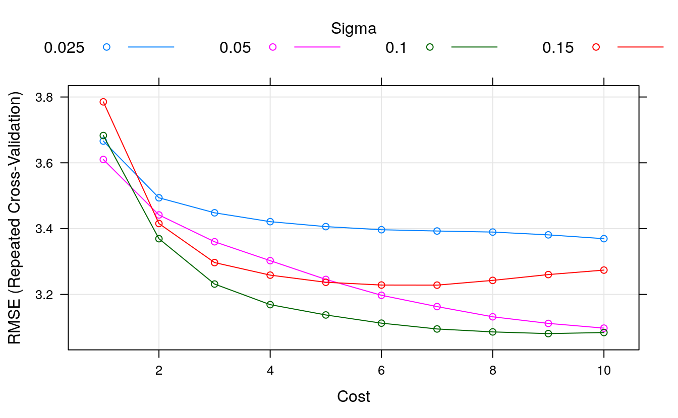
33.8 Ensembling
We can try some ensemble methods on the problem and see if we can get a further decrease in our RMSE.
- Random Forest, bagging (RF).
- Gradient Boosting Machines (GBM).
- Cubist, boosting (CUBIST).
# try ensembles
seed <- 7
trainControl <- trainControl(method="repeatedcv", number=10, repeats=3)
metric <- "RMSE"

# Random Forest
set.seed(seed)
fit.rf <- train(medv~., data=dataset, method="rf", metric=metric,
                preProc=c("BoxCox"),
                trControl=trainControl)

# Stochastic Gradient Boosting
set.seed(seed)
fit.gbm <- train(medv~., data=dataset, method="gbm", metric=metric,
                 preProc=c("BoxCox"),
                 trControl=trainControl, verbose=FALSE)
# Cubist
set.seed(seed)
fit.cubist <- train(medv~., data=dataset, method="cubist", metric=metric,
                    preProc=c("BoxCox"), trControl=trainControl)
# Compare algorithms
ensembleResults <- resamples(list(RF  = fit.rf,
                                  GBM = fit.gbm,
                                  CUBIST = fit.cubist))
summary(ensembleResults)
#>
#> Call:
#> summary.resamples(object = ensembleResults)
#>
#> Models: RF, GBM, CUBIST
#> Number of resamples: 30
#>
#> MAE
#>        Min. 1st Qu. Median Mean 3rd Qu. Max. NA's
#> RF     1.64    1.98   2.20 2.21    2.30 3.22    0
#> GBM    1.65    1.98   2.27 2.33    2.55 3.75    0
#> CUBIST 1.31    1.75   1.95 2.00    2.17 2.89    0
#>
#> RMSE
#>        Min. 1st Qu. Median Mean 3rd Qu. Max. NA's
#> RF     2.11    2.58   3.08 3.22    3.70 6.52    0
#> GBM    1.92    2.54   3.31 3.38    3.67 6.85    0
#> CUBIST 1.79    2.38   2.74 3.09    3.78 5.79    0
#>
#> Rsquared
#>         Min. 1st Qu. Median  Mean 3rd Qu.  Max. NA's
#> RF     0.597   0.852  0.900 0.869   0.919 0.972    0
#> GBM    0.558   0.815  0.889 0.851   0.912 0.964    0
#> CUBIST 0.681   0.818  0.909 0.875   0.932 0.970    0
dotplot(ensembleResults)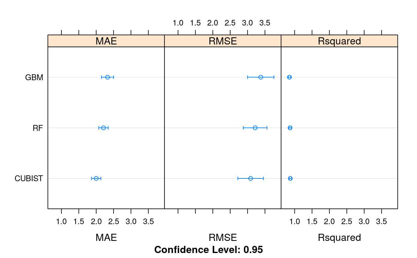
Let’s dive deeper into Cubist and see if we can tune it further and get more skill out of it. Cubist has two parameters that are tunable with caret: committees which is the number of boosting operations and neighbors which is used during prediction and is the number of instances used to correct the rule-based prediction (although the documentation is perhaps a little ambiguous on this).
# look at parameters used for Cubist
print(fit.cubist)
#> Cubist
#>
#> 407 samples
#>  13 predictor
#>
#> Pre-processing: Box-Cox transformation (11)
#> Resampling: Cross-Validated (10 fold, repeated 3 times)
#> Summary of sample sizes: 365, 366, 366, 367, 366, 366, ...
#> Resampling results across tuning parameters:
#>
#>   committees  neighbors  RMSE  Rsquared  MAE
#>    1          0          3.94  0.805     2.50
#>    1          5          3.66  0.828     2.24
#>    1          9          3.69  0.825     2.26
#>   10          0          3.45  0.848     2.29
#>   10          5          3.19  0.868     2.04
#>   10          9          3.23  0.864     2.07
#>   20          0          3.34  0.858     2.25
#>   20          5          3.09  0.875     2.00
#>   20          9          3.12  0.872     2.03
#>
#> RMSE was used to select the optimal model using the smallest value.
#> The final values used for the model were committees = 20 and neighbors = 5.
Let’s use a grid search to tune around those values. We’ll try all committees between 15 and 25 and spot-check a neighbors value above and below 5.
library(Cubist)
# Tune the Cubist algorithm
trainControl <- trainControl(method="repeatedcv", number=10, repeats=3)
metric <- "RMSE"
set.seed(7)
grid <- expand.grid(.committees = seq(15, 25, by=1),
                    .neighbors = c(3, 5, 7))

tune.cubist <- train(medv~., data=dataset, method = "cubist", metric=metric,
                     preProc=c("BoxCox"),
                     tuneGrid=grid, trControl=trainControl)
print(tune.cubist)
#> Cubist
#>
#> 407 samples
#>  13 predictor
#>
#> Pre-processing: Box-Cox transformation (11)
#> Resampling: Cross-Validated (10 fold, repeated 3 times)
#> Summary of sample sizes: 365, 366, 366, 367, 366, 366, ...
#> Resampling results across tuning parameters:
#>
#>   committees  neighbors  RMSE  Rsquared  MAE
#>   15          3          3.07  0.877     2.00
#>   15          5          3.13  0.873     2.02
#>   15          7          3.14  0.871     2.03
#>   16          3          3.05  0.878     1.99
#>   16          5          3.11  0.874     2.01
#>   16          7          3.12  0.872     2.02
#>   17          3          3.04  0.879     1.98
#>   17          5          3.09  0.875     2.00
#>   17          7          3.11  0.873     2.01
#>   18          3          3.03  0.880     1.97
#>   18          5          3.08  0.876     2.00
#>   18          7          3.10  0.874     2.01
#>   19          3          3.03  0.880     1.97
#>   19          5          3.08  0.876     1.99
#>   19          7          3.10  0.874     2.01
#>   20          3          3.03  0.879     1.98
#>   20          5          3.09  0.875     2.00
#>   20          7          3.10  0.874     2.01
#>   21          3          3.03  0.879     1.98
#>   21          5          3.09  0.876     2.00
#>   21          7          3.10  0.874     2.02
#>   22          3          3.03  0.879     1.98
#>   22          5          3.09  0.875     2.00
#>   22          7          3.10  0.874     2.02
#>   23          3          3.03  0.880     1.98
#>   23          5          3.09  0.876     2.01
#>   23          7          3.10  0.874     2.02
#>   24          3          3.03  0.879     1.98
#>   24          5          3.09  0.875     2.01
#>   24          7          3.11  0.873     2.02
#>   25          3          3.03  0.880     1.98
#>   25          5          3.09  0.876     2.01
#>   25          7          3.10  0.874     2.02
#>
#> RMSE was used to select the optimal model using the smallest value.
#> The final values used for the model were committees = 25 and neighbors = 3.
plot(tune.cubist)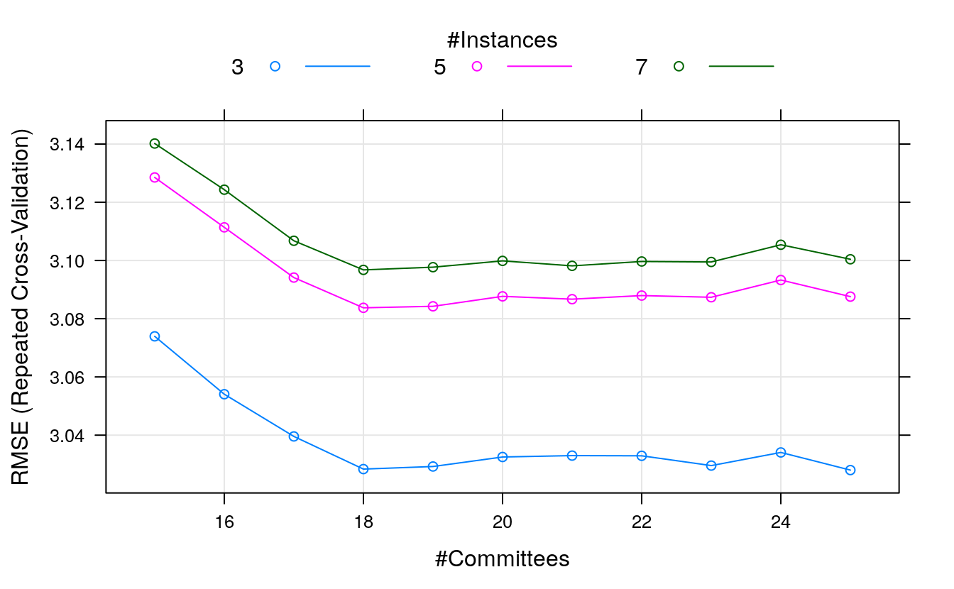
We can see that we have achieved a more accurate model again with an RMSE of 2.822 using committees = 18 and neighbors = 3.
It looks like the results for the Cubist algorithm are the most accurate. Let’s finalize it by creating a new standalone Cubist model with the parameters above trained using the whole dataset. We must also use the Box-Cox power transform.
33.9 Finalize the model
# prepare the data transform using training data
set.seed(7)
x <- dataset[,1:13]
y <- dataset[,14]

# transform
preprocessParams <- preProcess(x, method=c("BoxCox"))
transX <- predict(preprocessParams, x)

# train the final model
finalModel <- cubist(x = transX, y=y, committees=18)
summary(finalModel)
#>
#> Call:
#> cubist.default(x = transX, y = y, committees = 18)
#>
#>
#> Cubist [Release 2.07 GPL Edition]  Fri Nov 20 00:39:24 2020
#> ---------------------------------
#>
#>     Target attribute `outcome'
#>
#> Read 407 cases (14 attributes) from undefined.data
#>
#> Model 1:
#>
#>   Rule 1/1: [84 cases, mean 14.29, range 5 to 27.5, est err 1.97]
#>
#>     if
#>  nox > -0.4864544
#>     then
#>  outcome = 35.08 - 2.45 crim - 4.31 lstat + 2.1e-05 b
#>
#>   Rule 1/2: [163 cases, mean 19.37, range 7 to 31, est err 2.10]
#>
#>     if
#>  nox <= -0.4864544
#>  lstat > 2.848535
#>     then
#>  outcome = 186.8 - 2.34 lstat - 3.3 dis - 88 tax + 2 rad + 4.4 rm
#>            - 0.033 ptratio - 0.0116 age + 3.3e-05 b
#>
#>   Rule 1/3: [24 cases, mean 21.65, range 18.2 to 25.3, est err 1.19]
#>
#>     if
#>  rm <= 3.326479
#>  dis > 1.345056
#>  lstat <= 2.848535
#>     then
#>  outcome = 43.83 + 14.5 rm - 2.29 lstat - 3.8 dis - 30 tax
#>            - 0.014 ptratio - 1.4 nox + 0.017 zn + 0.4 rad + 0.15 crim
#>            - 0.0025 age + 8e-06 b
#>
#>   Rule 1/4: [7 cases, mean 27.66, range 20.7 to 50, est err 7.89]
#>
#>     if
#>  rm > 3.326479
#>  ptratio > 193.545
#>  lstat <= 2.848535
#>     then
#>  outcome = 19.64 + 7.8 rm - 3.4 dis - 1.62 lstat + 0.27 crim - 0.006 age
#>            + 0.023 zn - 7 tax - 0.003 ptratio
#>
#>   Rule 1/5: [141 cases, mean 30.60, range 15 to 50, est err 2.09]
#>
#>     if
#>  rm > 3.326479
#>  ptratio <= 193.545
#>     then
#>  outcome = 137.95 + 21.7 rm - 3.43 lstat - 4.9 dis - 87 tax - 0.0162 age
#>            - 0.039 ptratio + 0.06 crim + 0.005 zn
#>
#>   Rule 1/6: [8 cases, mean 32.16, range 22.1 to 50, est err 8.67]
#>
#>     if
#>  rm <= 3.326479
#>  dis <= 1.345056
#>  lstat <= 2.848535
#>     then
#>  outcome = -19.71 + 18.58 lstat - 15.9 dis + 5.6 rm
#>
#> Model 2:
#>
#>   Rule 2/1: [23 cases, mean 10.57, range 5 to 15, est err 3.06]
#>
#>     if
#>  crim > 2.086391
#>  dis <= 0.6604174
#>  b > 67032.41
#>     then
#>  outcome = 37.22 - 4.83 crim - 7 dis - 1.9 lstat - 1.9e-05 b - 0.7 rm
#>
#>   Rule 2/2: [70 cases, mean 14.82, range 5 to 50, est err 3.90]
#>
#>     if
#>  rm <= 3.620525
#>  dis <= 0.6604174
#>     then
#>  outcome = 74.6 - 21 dis - 5.09 lstat - 15 tax - 0.0017 age + 6e-06 b
#>
#>   Rule 2/3: [18 cases, mean 18.03, range 7.5 to 50, est err 6.81]
#>
#>     if
#>  crim > 2.086391
#>  dis <= 0.6604174
#>  b <= 67032.41
#>     then
#>  outcome = 94.95 - 40.1 dis - 8.15 crim - 7.14 lstat - 3.5e-05 b - 1.3 rm
#>
#>   Rule 2/4: [258 cases, mean 20.74, range 9.5 to 36.2, est err 1.92]
#>
#>     if
#>  rm <= 3.620525
#>  dis > 0.6604174
#>  lstat > 1.805082
#>     then
#>  outcome = 61.89 - 2.56 lstat + 5.5 rm - 2.8 dis + 7.3e-05 b - 0.0132 age
#>            - 26 tax - 0.11 indus - 0.004 ptratio + 0.05 crim
#>
#>   Rule 2/5: [37 cases, mean 31.66, range 10.4 to 50, est err 3.70]
#>
#>     if
#>  rm > 3.620525
#>  lstat > 1.805082
#>     then
#>  outcome = 370.03 - 180 tax - 2.19 lstat - 1.7 dis + 2.6 rm
#>            - 0.016 ptratio - 0.25 indus + 0.12 crim - 0.0021 age
#>            + 9e-06 b - 0.5 nox
#>
#>   Rule 2/6: [42 cases, mean 38.23, range 22.8 to 50, est err 3.70]
#>
#>     if
#>  lstat <= 1.805082
#>     then
#>  outcome = -73.87 + 32.4 rm - 9.4e-05 b - 1.8 dis + 0.028 zn
#>            - 0.013 ptratio
#>
#>   Rule 2/7: [4 cases, mean 40.20, range 37.6 to 42.8, est err 7.33]
#>
#>     if
#>  rm > 4.151791
#>  dis > 1.114486
#>     then
#>  outcome = 35.8
#>
#>   Rule 2/8: [8 cases, mean 47.45, range 41.3 to 50, est err 10.01]
#>
#>     if
#>  dis <= 1.114486
#>  lstat <= 1.805082
#>     then
#>  outcome = 48.96 + 7.53 crim - 4.1e-05 b - 0.8 dis + 1.2 rm + 0.008 zn
#>
#> Model 3:
#>
#>   Rule 3/1: [81 cases, mean 13.93, range 5 to 23.2, est err 2.24]
#>
#>     if
#>  nox > -0.4864544
#>  lstat > 2.848535
#>     then
#>  outcome = 55.03 - 0.0631 age - 2.11 crim + 12 nox - 4.16 lstat
#>            + 3.2e-05 b
#>
#>   Rule 3/2: [163 cases, mean 19.37, range 7 to 31, est err 2.29]
#>
#>     if
#>  nox <= -0.4864544
#>  lstat > 2.848535
#>     then
#>  outcome = 77.73 - 0.059 ptratio + 5.8 rm - 3.2 dis - 0.0139 age
#>            - 1.15 lstat - 30 tax - 1.1 nox + 0.4 rad
#>
#>   Rule 3/3: [62 cases, mean 24.01, range 18.2 to 50, est err 3.56]
#>
#>     if
#>  rm <= 3.448196
#>  lstat <= 2.848535
#>     then
#>  outcome = 94.86 + 18.2 rm + 0.63 crim - 68 tax - 2.3 dis - 3 nox
#>            - 0.0098 age - 0.41 indus - 0.011 ptratio
#>
#>   Rule 3/4: [143 cases, mean 28.76, range 16.5 to 50, est err 2.53]
#>
#>     if
#>  dis > 0.9547035
#>  lstat <= 2.848535
#>     then
#>  outcome = 269.46 + 17.9 rm - 6.1 dis - 153 tax + 0.96 crim - 0.0217 age
#>            - 5.5 nox - 0.62 indus - 0.028 ptratio - 0.89 lstat + 0.4 rad
#>            + 0.004 zn
#>
#>   Rule 3/5: [10 cases, mean 35.13, range 21.9 to 50, est err 9.31]
#>
#>     if
#>  dis <= 0.6492998
#>  lstat <= 2.848535
#>     then
#>  outcome = 58.69 - 56.8 dis - 8.4 nox
#>
#>   Rule 3/6: [10 cases, mean 41.67, range 22 to 50, est err 9.89]
#>
#>     if
#>  dis > 0.6492998
#>  dis <= 0.9547035
#>  lstat <= 2.848535
#>     then
#>  outcome = 47.93
#>
#> Model 4:
#>
#>   Rule 4/1: [69 cases, mean 12.69, range 5 to 27.5, est err 2.55]
#>
#>     if
#>  dis <= 0.719156
#>  lstat > 3.508535
#>     then
#>  outcome = 180.13 - 7.2 dis + 0.039 age - 3.78 lstat - 83 tax
#>
#>   Rule 4/2: [164 cases, mean 19.42, range 12 to 31, est err 1.96]
#>
#>     if
#>  dis > 0.719156
#>  lstat > 2.848535
#>     then
#>  outcome = 52.75 + 7.1 rm - 2.05 lstat - 3.6 dis + 8.2e-05 b - 0.0152 age
#>            - 25 tax + 0.5 rad - 1.2 nox - 0.008 ptratio
#>
#>   Rule 4/3: [11 cases, mean 20.39, range 15 to 27.9, est err 3.51]
#>
#>     if
#>  dis <= 0.719156
#>  lstat > 2.848535
#>  lstat <= 3.508535
#>     then
#>  outcome = 21.69
#>
#>   Rule 4/4: [63 cases, mean 23.22, range 16.5 to 31.5, est err 1.67]
#>
#>     if
#>  rm <= 3.483629
#>  dis > 0.9731624
#>  lstat <= 2.848535
#>     then
#>  outcome = 59.35 - 3.96 lstat - 3.1 dis + 1 rm - 14 tax + 0.3 rad
#>            - 0.7 nox - 0.005 ptratio + 6e-06 b
#>
#>   Rule 4/5: [8 cases, mean 33.08, range 22 to 50, est err 23.91]
#>
#>     if
#>  rm > 3.369183
#>  dis <= 0.9731624
#>  lstat > 2.254579
#>  lstat <= 2.848535
#>     then
#>  outcome = -322.28 + 64.9 lstat + 56.8 rm - 30.2 dis
#>
#>   Rule 4/6: [7 cases, mean 33.87, range 22.1 to 50, est err 13.21]
#>
#>     if
#>  rm <= 3.369183
#>  dis <= 0.9731624
#>  lstat <= 2.848535
#>     then
#>  outcome = -52.11 + 43.45 lstat - 30.8 dis
#>
#>   Rule 4/7: [91 cases, mean 34.43, range 21.9 to 50, est err 3.32]
#>
#>     if
#>  rm > 3.483629
#>  lstat <= 2.848535
#>     then
#>  outcome = -33.09 + 22 rm - 5.02 lstat - 0.038 ptratio - 0.9 dis
#>            + 0.005 zn
#>
#>   Rule 4/8: [22 cases, mean 36.99, range 21.9 to 50, est err 13.21]
#>
#>     if
#>  dis <= 0.9731624
#>  lstat <= 2.848535
#>     then
#>  outcome = 80.3 - 17.43 lstat - 0.134 ptratio + 2.5 rm - 1.2 dis
#>            + 0.008 zn
#>
#> Model 5:
#>
#>   Rule 5/1: [84 cases, mean 14.29, range 5 to 27.5, est err 2.81]
#>
#>     if
#>  nox > -0.4864544
#>     then
#>  outcome = 56.48 + 28.5 nox - 0.0875 age - 3.58 crim - 5.9 dis
#>            - 2.96 lstat + 0.073 ptratio + 1.7e-05 b
#>
#>   Rule 5/2: [163 cases, mean 19.37, range 7 to 31, est err 2.38]
#>
#>     if
#>  nox <= -0.4864544
#>  lstat > 2.848535
#>     then
#>  outcome = 61.59 - 0.064 ptratio + 5.9 rm - 3.1 dis - 0.0142 age
#>            - 0.77 lstat - 21 tax
#>
#>   Rule 5/3: [163 cases, mean 29.94, range 16.5 to 50, est err 3.65]
#>
#>     if
#>  lstat <= 2.848535
#>     then
#>  outcome = 264.17 + 21.9 rm - 8 dis - 155 tax - 0.0317 age
#>            - 0.032 ptratio + 0.29 crim - 1.6 nox - 0.25 indus
#>
#>   Rule 5/4: [10 cases, mean 35.13, range 21.9 to 50, est err 11.79]
#>
#>     if
#>  dis <= 0.6492998
#>  lstat <= 2.848535
#>     then
#>  outcome = 68.19 - 73.4 dis + 1.1 rm + 0.11 crim - 0.6 nox - 0.1 indus
#>            - 0.0017 age - 0.12 lstat
#>
#> Model 6:
#>
#>   Rule 6/1: [71 cases, mean 15.57, range 5 to 50, est err 4.42]
#>
#>     if
#>  dis <= 0.6443245
#>  lstat > 1.793385
#>     then
#>  outcome = 45.7 - 20.6 dis - 5.38 lstat
#>
#>   Rule 6/2: [159 cases, mean 19.53, range 8.3 to 36.2, est err 2.08]
#>
#>     if
#>  rm <= 3.329365
#>  dis > 0.6443245
#>     then
#>  outcome = 24.33 + 8.8 rm + 0.000118 b - 0.0146 age - 2.5 dis
#>            - 0.95 lstat + 0.37 crim - 0.32 indus + 0.02 zn - 16 tax
#>            + 0.2 rad - 0.5 nox - 0.004 ptratio
#>
#>   Rule 6/3: [175 cases, mean 27.80, range 9.5 to 50, est err 2.95]
#>
#>     if
#>  rm > 3.329365
#>  dis > 0.6443245
#>     then
#>  outcome = 0.11 + 18.7 rm - 3.11 lstat + 8.1e-05 b - 1.1 dis + 0.19 crim
#>            - 20 tax - 0.19 indus + 0.3 rad - 0.7 nox - 0.005 ptratio
#>            + 0.006 zn
#>
#>   Rule 6/4: [8 cases, mean 32.50, range 21.9 to 50, est err 10.34]
#>
#>     if
#>  dis <= 0.6443245
#>  lstat > 1.793385
#>  lstat <= 2.894121
#>     then
#>  outcome = 69.38 - 71.2 dis - 0.14 lstat
#>
#>   Rule 6/5: [34 cases, mean 37.55, range 22.8 to 50, est err 3.55]
#>
#>     if
#>  rm <= 4.151791
#>  lstat <= 1.793385
#>     then
#>  outcome = -125.14 + 41.7 rm + 4.3 rad + 1.48 indus - 0.014 ptratio
#>
#>   Rule 6/6: [7 cases, mean 43.66, range 37.6 to 50, est err 3.12]
#>
#>     if
#>  rm > 4.151791
#>  lstat <= 1.793385
#>     then
#>  outcome = -137.67 + 44.6 rm - 0.064 ptratio
#>
#> Model 7:
#>
#>   Rule 7/1: [84 cases, mean 14.29, range 5 to 27.5, est err 2.91]
#>
#>     if
#>  nox > -0.4864544
#>     then
#>  outcome = 46.85 - 3.45 crim - 0.0621 age + 14.2 nox + 4.4 dis
#>            - 2.01 lstat + 2.5e-05 b
#>
#>   Rule 7/2: [323 cases, mean 24.66, range 7 to 50, est err 3.68]
#>
#>     if
#>  nox <= -0.4864544
#>     then
#>  outcome = 57.59 - 0.065 ptratio - 4.4 dis + 6.8 rm - 0.0143 age
#>            - 1.36 lstat - 19 tax - 0.8 nox - 0.12 crim + 0.09 indus
#>
#>   Rule 7/3: [132 cases, mean 28.24, range 16.5 to 50, est err 2.55]
#>
#>     if
#>  dis > 1.063503
#>  lstat <= 2.848535
#>     then
#>  outcome = 270.92 + 24.5 rm - 0.0418 age - 165 tax - 5.7 dis
#>            - 0.028 ptratio + 0.26 crim + 0.017 zn
#>
#>   Rule 7/4: [7 cases, mean 36.01, range 23.3 to 50, est err 3.87]
#>
#>     if
#>  dis <= 0.6002641
#>  lstat <= 2.848535
#>     then
#>  outcome = 57.18 - 69.5 dis - 6.5 nox + 1.9 rm - 0.015 ptratio
#>
#>   Rule 7/5: [24 cases, mean 37.55, range 21.9 to 50, est err 8.66]
#>
#>     if
#>  dis > 0.6002641
#>  dis <= 1.063503
#>  lstat <= 2.848535
#>     then
#>  outcome = -3.76 - 14.8 dis - 2.93 crim - 0.16 ptratio + 17.5 rm - 15 nox
#>
#> Model 8:
#>
#>   Rule 8/1: [80 cases, mean 13.75, range 5 to 27.9, est err 3.51]
#>
#>     if
#>  dis <= 0.719156
#>  lstat > 2.848535
#>     then
#>  outcome = 123.46 - 11.3 dis - 5.06 lstat - 45 tax + 0.9 rad + 1.7e-05 b
#>
#>   Rule 8/2: [164 cases, mean 19.42, range 12 to 31, est err 2.05]
#>
#>     if
#>  dis > 0.719156
#>  lstat > 2.848535
#>     then
#>  outcome = 227.11 - 120 tax + 6.4 rm + 9.3e-05 b - 3.3 dis + 2 rad
#>            - 0.0183 age - 0.93 lstat + 0.05 crim - 0.3 nox
#>
#>   Rule 8/3: [163 cases, mean 29.94, range 16.5 to 50, est err 3.54]
#>
#>     if
#>  lstat <= 2.848535
#>     then
#>  outcome = 158.14 - 5.73 lstat + 10.8 rm - 4 dis - 83 tax - 4.1 nox
#>            + 0.61 crim - 0.54 indus + 1 rad + 3.6e-05 b
#>
#>   Rule 8/4: [7 cases, mean 36.01, range 23.3 to 50, est err 11.44]
#>
#>     if
#>  dis <= 0.6002641
#>  lstat <= 2.848535
#>     then
#>  outcome = 72.89 - 87.2 dis + 0.6 rm - 0.13 lstat
#>
#>   Rule 8/5: [47 cases, mean 38.44, range 15 to 50, est err 5.71]
#>
#>     if
#>  rm > 3.726352
#>     then
#>  outcome = 602.95 - 10.4 lstat + 21 rm - 326 tax - 0.093 ptratio
#>
#> Model 9:
#>
#>   Rule 9/1: [81 cases, mean 13.93, range 5 to 23.2, est err 2.91]
#>
#>     if
#>  nox > -0.4864544
#>  lstat > 2.848535
#>     then
#>  outcome = 41.11 - 3.98 crim - 4.42 lstat + 6.7 nox
#>
#>   Rule 9/2: [163 cases, mean 19.37, range 7 to 31, est err 2.49]
#>
#>     if
#>  nox <= -0.4864544
#>  lstat > 2.848535
#>     then
#>  outcome = 44.98 - 0.068 ptratio - 4.4 dis + 6.6 rm - 1.25 lstat
#>            - 0.0118 age - 0.9 nox - 12 tax - 0.08 crim + 0.06 indus
#>
#>   Rule 9/3: [132 cases, mean 28.24, range 16.5 to 50, est err 2.35]
#>
#>     if
#>  dis > 1.063503
#>  lstat <= 2.848535
#>     then
#>  outcome = 157.67 + 22.2 rm - 0.0383 age - 104 tax - 0.033 ptratio
#>            - 2.2 dis
#>
#>   Rule 9/4: [7 cases, mean 30.76, range 21.9 to 50, est err 6.77]
#>
#>     if
#>  dis <= 1.063503
#>  b <= 66469.73
#>  lstat <= 2.848535
#>     then
#>  outcome = 48.52 - 56.1 dis - 12.9 nox - 0.032 ptratio + 2.7 rm
#>
#>   Rule 9/5: [24 cases, mean 39.09, range 22 to 50, est err 6.20]
#>
#>     if
#>  dis <= 1.063503
#>  b > 66469.73
#>  lstat <= 2.848535
#>     then
#>  outcome = -5.49 - 34.8 dis - 20.7 nox + 18.2 rm - 0.051 ptratio
#>
#> Model 10:
#>
#>   Rule 10/1: [327 cases, mean 19.45, range 5 to 50, est err 2.77]
#>
#>     if
#>  rm <= 3.617282
#>  lstat > 1.805082
#>     then
#>  outcome = 270.78 - 4.09 lstat - 131 tax + 2.9 rad + 5.3e-05 b - 0.6 dis
#>            - 0.16 indus + 0.7 rm - 0.3 nox
#>
#>   Rule 10/2: [38 cases, mean 31.57, range 10.4 to 50, est err 4.71]
#>
#>     if
#>  rm > 3.617282
#>  lstat > 1.805082
#>     then
#>  outcome = 308.44 - 150 tax - 2.63 lstat + 1.6 rad - 1.9 dis - 0.49 indus
#>            + 2.5 rm + 3e-05 b - 1.2 nox + 0.14 crim - 0.005 ptratio
#>
#>   Rule 10/3: [35 cases, mean 37.15, range 22.8 to 50, est err 2.76]
#>
#>     if
#>  rm <= 4.151791
#>  lstat <= 1.805082
#>     then
#>  outcome = -71.65 + 33.4 rm - 0.017 ptratio - 0.34 lstat + 0.2 rad
#>            - 0.3 dis - 7 tax - 0.4 nox
#>
#>   Rule 10/4: [10 cases, mean 42.63, range 21.9 to 50, est err 7.11]
#>
#>     if
#>  rm > 4.151791
#>     then
#>  outcome = -92.51 + 32.8 rm - 0.03 ptratio
#>
#> Model 11:
#>
#>   Rule 11/1: [84 cases, mean 14.29, range 5 to 27.5, est err 4.13]
#>
#>     if
#>  nox > -0.4864544
#>     then
#>  outcome = 42.75 - 4.12 crim + 18.1 nox - 0.045 age + 6.8 dis
#>            - 1.86 lstat
#>
#>   Rule 11/2: [244 cases, mean 17.56, range 5 to 31, est err 4.29]
#>
#>     if
#>  lstat > 2.848535
#>     then
#>  outcome = 34.83 - 5.2 dis - 0.058 ptratio - 0.0228 age + 5.8 rm
#>            - 0.56 lstat - 0.07 crim - 0.4 nox - 5 tax
#>
#>   Rule 11/3: [163 cases, mean 29.94, range 16.5 to 50, est err 3.49]
#>
#>     if
#>  lstat <= 2.848535
#>     then
#>  outcome = 151.5 + 23.3 rm - 5.5 dis + 1.01 crim - 0.0211 age
#>            - 0.052 ptratio - 98 tax + 0.031 zn
#>
#>   Rule 11/4: [10 cases, mean 35.13, range 21.9 to 50, est err 25.19]
#>
#>     if
#>  dis <= 0.6492998
#>  lstat <= 2.848535
#>     then
#>  outcome = 130.87 - 157.1 dis - 15.76 crim
#>
#> Model 12:
#>
#>   Rule 12/1: [80 cases, mean 13.75, range 5 to 27.9, est err 4.76]
#>
#>     if
#>  dis <= 0.719156
#>  lstat > 2.894121
#>     then
#>  outcome = 182.68 - 6.03 lstat - 7.6 dis - 76 tax + 1.3 rad - 0.52 indus
#>            + 2.6e-05 b
#>
#>   Rule 12/2: [300 cases, mean 19.10, range 5 to 50, est err 2.76]
#>
#>     if
#>  rm <= 3.50716
#>  lstat > 1.793385
#>     then
#>  outcome = 83.61 - 3 lstat + 9.6e-05 b - 0.0072 age - 33 tax + 0.7 rad
#>            + 0.32 indus
#>
#>   Rule 12/3: [10 cases, mean 24.25, range 15.7 to 36.2, est err 13.88]
#>
#>     if
#>  rm <= 3.50716
#>  tax <= 1.865769
#>     then
#>  outcome = 35.46
#>
#>   Rule 12/4: [10 cases, mean 32.66, range 21.9 to 50, est err 6.28]
#>
#>     if
#>  dis <= 0.719156
#>  lstat > 1.793385
#>  lstat <= 2.894121
#>     then
#>  outcome = 82.78 - 69.5 dis - 3.66 indus
#>
#>   Rule 12/5: [89 cases, mean 32.75, range 13.4 to 50, est err 3.39]
#>
#>     if
#>  rm > 3.50716
#>  dis > 0.719156
#>     then
#>  outcome = 313.22 + 13.7 rm - 174 tax - 3.06 lstat + 4.8e-05 b - 1.5 dis
#>            - 0.41 indus + 0.7 rad - 0.0055 age + 0.22 crim
#>
#>   Rule 12/6: [34 cases, mean 37.55, range 22.8 to 50, est err 3.25]
#>
#>     if
#>  rm <= 4.151791
#>  lstat <= 1.793385
#>     then
#>  outcome = -86.8 + 36 rm - 0.3 lstat - 5 tax
#>
#>   Rule 12/7: [7 cases, mean 43.66, range 37.6 to 50, est err 5.79]
#>
#>     if
#>  rm > 4.151791
#>  lstat <= 1.793385
#>     then
#>  outcome = -158.68 + 47.4 rm - 0.02 ptratio
#>
#> Model 13:
#>
#>   Rule 13/1: [84 cases, mean 14.29, range 5 to 27.5, est err 2.87]
#>
#>     if
#>  nox > -0.4864544
#>     then
#>  outcome = 54.69 - 3.79 crim - 0.0644 age + 11.4 nox - 2.53 lstat
#>
#>   Rule 13/2: [8 cases, mean 17.76, range 7 to 27.9, est err 13.69]
#>
#>     if
#>  nox <= -0.4864544
#>  age > 296.3423
#>  b <= 60875.57
#>     then
#>  outcome = -899.55 + 3.0551 age
#>
#>   Rule 13/3: [31 cases, mean 17.94, range 7 to 27.9, est err 5.15]
#>
#>     if
#>  nox <= -0.4864544
#>  b <= 60875.57
#>  lstat > 2.848535
#>     then
#>  outcome = 44.43 - 3.51 lstat - 0.054 ptratio - 1.4 dis - 0.26 crim
#>            - 0.0042 age - 0.21 indus + 0.9 rm
#>
#>   Rule 13/4: [163 cases, mean 19.37, range 7 to 31, est err 3.37]
#>
#>     if
#>  nox <= -0.4864544
#>  lstat > 2.848535
#>     then
#>  outcome = -5.76 + 0.000242 b + 8.9 rm - 5.2 dis - 0.0209 age
#>            - 0.042 ptratio - 0.63 indus
#>
#>   Rule 13/5: [163 cases, mean 29.94, range 16.5 to 50, est err 3.45]
#>
#>     if
#>  lstat <= 2.848535
#>     then
#>  outcome = 178.84 + 23.8 rm - 0.0343 age - 4.5 dis - 114 tax + 0.88 crim
#>            - 0.048 ptratio + 0.026 zn
#>
#>   Rule 13/6: [7 cases, mean 36.01, range 23.3 to 50, est err 14.09]
#>
#>     if
#>  dis <= 0.6002641
#>  lstat <= 2.848535
#>     then
#>  outcome = 45.82 - 70.3 dis - 9.9 nox + 5.1 rm + 1.5 rad
#>
#>   Rule 13/7: [31 cases, mean 37.21, range 21.9 to 50, est err 7.73]
#>
#>     if
#>  dis <= 1.063503
#>  lstat <= 2.848535
#>     then
#>  outcome = 95.05 - 4.52 lstat - 7.5 dis + 8.8 rm - 0.064 ptratio
#>            - 6.2 nox - 36 tax
#>
#> Model 14:
#>
#>   Rule 14/1: [49 cases, mean 16.06, range 8.4 to 22.7, est err 3.17]
#>
#>     if
#>  nox > -0.4205732
#>  lstat > 2.848535
#>     then
#>  outcome = 12.83 + 42.3 nox - 4.77 lstat + 9.7 rm + 7.8e-05 b
#>
#>   Rule 14/2: [78 cases, mean 16.36, range 5 to 50, est err 5.17]
#>
#>     if
#>  dis <= 0.6604174
#>     then
#>  outcome = 110.6 - 10.4 dis - 4.85 lstat + 0.0446 age - 46 tax + 0.8 rad
#>
#>   Rule 14/3: [57 cases, mean 18.40, range 9.5 to 31, est err 2.43]
#>
#>     if
#>  nox > -0.9365134
#>  nox <= -0.4205732
#>  age > 245.2507
#>  dis > 0.6604174
#>  lstat > 2.848535
#>     then
#>  outcome = 206.69 - 0.1012 age - 7.05 lstat + 12.2 nox - 67 tax + 0.3 rad
#>            + 0.5 rm - 0.3 dis
#>
#>   Rule 14/4: [230 cases, mean 20.19, range 9.5 to 36.2, est err 2.09]
#>
#>     if
#>  rm <= 3.483629
#>  dis > 0.6492998
#>     then
#>  outcome = 119.15 - 2.61 lstat + 5.2 rm - 57 tax - 1.8 dis - 2.4 nox
#>            + 0.7 rad + 0.24 crim + 0.003 age - 0.007 ptratio + 9e-06 b
#>
#>   Rule 14/5: [48 cases, mean 20.28, range 10.2 to 24.5, est err 2.13]
#>
#>     if
#>  nox > -0.9365134
#>  nox <= -0.4205732
#>  age <= 245.2507
#>  dis > 0.6604174
#>  lstat > 2.848535
#>     then
#>  outcome = 19.4 - 1.91 lstat + 1.02 indus - 0.013 age + 2.7 rm + 2.6 nox
#>            - 0.009 ptratio
#>
#>   Rule 14/6: [44 cases, mean 20.69, range 14.4 to 29.6, est err 2.26]
#>
#>     if
#>  nox <= -0.9365134
#>  lstat > 2.848535
#>     then
#>  outcome = 87.55 - 0.000315 b - 6.5 dis + 2.6 rad - 0.59 lstat - 18 tax
#>
#>   Rule 14/7: [102 cases, mean 32.44, range 13.4 to 50, est err 3.35]
#>
#>     if
#>  rm > 3.483629
#>  dis > 0.6492998
#>     then
#>  outcome = 126.92 + 22.7 rm - 4.68 lstat - 85 tax - 0.036 ptratio
#>            - 1.1 dis + 0.007 zn
#>
#>   Rule 14/8: [84 cases, mean 33.40, range 21 to 50, est err 2.44]
#>
#>     if
#>  rm > 3.483629
#>  tax <= 1.896025
#>     then
#>  outcome = 347.12 + 25.2 rm - 213 tax - 3.5 lstat - 0.013 ptratio
#>
#>   Rule 14/9: [10 cases, mean 35.13, range 21.9 to 50, est err 12.13]
#>
#>     if
#>  dis <= 0.6492998
#>  lstat <= 2.848535
#>     then
#>  outcome = 72.65 - 77.8 dis
#>
#> Model 15:
#>
#>   Rule 15/1: [28 cases, mean 12.35, range 5 to 27.9, est err 4.09]
#>
#>     if
#>  crim > 2.405809
#>  b > 16084.5
#>     then
#>  outcome = 53.45 - 7.8 crim - 3.5 lstat - 0.0189 age
#>
#>   Rule 15/2: [11 cases, mean 13.56, range 8.3 to 27.5, est err 5.99]
#>
#>     if
#>  crim > 2.405809
#>  b <= 16084.5
#>     then
#>  outcome = 8.73 + 0.001756 b
#>
#>   Rule 15/3: [244 cases, mean 17.56, range 5 to 31, est err 2.73]
#>
#>     if
#>  lstat > 2.848535
#>     then
#>  outcome = 103.02 - 0.0251 age - 2.37 lstat - 3.5 dis + 6.8e-05 b + 4 rm
#>            - 0.035 ptratio - 41 tax - 0.25 crim
#>
#>   Rule 15/4: [131 cases, mean 28.22, range 16.5 to 50, est err 2.59]
#>
#>     if
#>  dis > 1.086337
#>  lstat <= 2.848535
#>     then
#>  outcome = 267.07 + 17.7 rm - 0.0421 age - 150 tax - 5.5 dis + 0.88 crim
#>            - 0.035 ptratio + 0.031 zn - 0.12 lstat - 0.3 nox
#>
#>   Rule 15/5: [13 cases, mean 33.08, range 22 to 50, est err 4.44]
#>
#>     if
#>  nox <= -0.7229691
#>  dis <= 1.086337
#>  lstat <= 2.848535
#>     then
#>  outcome = 148.52 - 0.002365 b - 85.9 nox - 1 dis + 0.16 crim + 0.8 rm
#>            + 0.007 zn - 0.0016 age - 7 tax - 0.003 ptratio
#>
#>   Rule 15/6: [7 cases, mean 36.01, range 23.3 to 50, est err 7.00]
#>
#>     if
#>  dis <= 0.6002641
#>  lstat <= 2.848535
#>     then
#>  outcome = 50.55 - 68.1 dis - 11.4 nox + 0.00012 b + 1 rm - 0.008 ptratio
#>
#>   Rule 15/7: [12 cases, mean 41.77, range 21.9 to 50, est err 9.73]
#>
#>     if
#>  nox > -0.7229691
#>  dis > 0.6002641
#>  lstat <= 2.848535
#>     then
#>  outcome = 13.74 - 92 nox - 40.5 dis - 0.023 ptratio + 2.6 rm
#>
#> Model 16:
#>
#>   Rule 16/1: [60 cases, mean 15.95, range 7.2 to 27.5, est err 3.16]
#>
#>     if
#>  nox > -0.4344906
#>     then
#>  outcome = 46.98 - 6.53 lstat - 6.9 dis - 1.1 rm
#>
#>   Rule 16/2: [45 cases, mean 16.89, range 5 to 50, est err 5.45]
#>
#>     if
#>  nox <= -0.4344906
#>  dis <= 0.6557049
#>     then
#>  outcome = 35.33 - 37 dis - 51.7 nox - 7.38 lstat - 0.4 rm
#>
#>   Rule 16/3: [128 cases, mean 19.97, range 9.5 to 36.2, est err 2.52]
#>
#>     if
#>  rm <= 3.626081
#>  dis > 0.6557049
#>  dis <= 1.298828
#>  lstat > 2.133251
#>     then
#>  outcome = 61.65 - 3.35 lstat + 4.9 dis + 1.6 rm - 1.3 nox - 22 tax
#>            + 0.5 rad + 1.8e-05 b + 0.09 crim - 0.004 ptratio
#>
#>   Rule 16/4: [140 cases, mean 21.93, range 12.7 to 35.1, est err 2.19]
#>
#>     if
#>  rm <= 3.626081
#>  dis > 1.298828
#>     then
#>  outcome = 54.16 - 3.58 lstat + 2.2 rad - 1.6 dis - 1.9 nox + 1.8 rm
#>            - 17 tax + 1.3e-05 b + 0.06 crim - 0.003 ptratio
#>
#>   Rule 16/5: [30 cases, mean 21.97, range 14.4 to 29.1, est err 2.41]
#>
#>     if
#>  rm <= 3.626081
#>  dis > 1.298828
#>  tax <= 1.879832
#>  lstat > 2.133251
#>     then
#>  outcome = -1065.35 + 566 tax + 8.7 rm - 0.13 lstat - 0.2 dis - 0.3 nox
#>
#>   Rule 16/6: [22 cases, mean 30.88, range 10.4 to 50, est err 4.51]
#>
#>     if
#>  rm > 3.626081
#>  lstat > 2.133251
#>     then
#>  outcome = 42.24 + 18.7 rm - 1.5 indus - 1.84 lstat - 2.5 nox - 1.6 dis
#>            - 39 tax + 0.7 rad - 0.012 ptratio + 0.0035 age + 1.2e-05 b
#>            + 0.11 crim
#>
#>   Rule 16/7: [73 cases, mean 34.52, range 20.6 to 50, est err 3.36]
#>
#>     if
#>  lstat <= 2.133251
#>     then
#>  outcome = 50.6 + 19.6 rm - 2.77 lstat - 3.2 nox - 1.7 dis - 45 tax
#>            + 1 rad + 0.007 age - 0.014 ptratio
#>
#> Model 17:
#>
#>   Rule 17/1: [116 cases, mean 15.37, range 5 to 27.9, est err 2.55]
#>
#>     if
#>  crim > 0.4779842
#>  lstat > 2.944963
#>     then
#>  outcome = 35.96 - 3.68 crim - 3.41 lstat + 0.3 nox
#>
#>   Rule 17/2: [112 cases, mean 19.13, range 7 to 31, est err 2.14]
#>
#>     if
#>  crim <= 0.4779842
#>  lstat > 2.944963
#>     then
#>  outcome = 184.65 - 0.0365 age + 9 rm - 4.1 dis - 97 tax + 8.4e-05 b
#>            - 0.024 ptratio
#>
#>   Rule 17/3: [9 cases, mean 28.37, range 15 to 50, est err 11.17]
#>
#>     if
#>  dis <= 0.9547035
#>  b <= 66469.73
#>  lstat <= 2.944963
#>     then
#>  outcome = -1.12 + 0.000454 b
#>
#>   Rule 17/4: [179 cases, mean 29.28, range 15 to 50, est err 3.35]
#>
#>     if
#>  lstat <= 2.944963
#>     then
#>  outcome = 278.16 + 20 rm - 7.4 dis - 0.0356 age - 161 tax + 0.051 zn
#>            - 0.61 lstat + 0.17 crim - 0.008 ptratio
#>
#>   Rule 17/5: [23 cases, mean 36.10, range 15 to 50, est err 10.83]
#>
#>     if
#>  dis <= 0.9547035
#>  lstat <= 2.944963
#>     then
#>  outcome = 233.74 - 8.5 dis + 12.1 rm + 1.15 crim - 2.42 lstat - 113 tax
#>            - 0.0221 age + 0.068 zn - 0.031 ptratio
#>
#> Model 18:
#>
#>   Rule 18/1: [84 cases, mean 14.29, range 5 to 27.5, est err 2.44]
#>
#>     if
#>  nox > -0.4864544
#>     then
#>  outcome = 41.55 - 6.2 lstat + 14.6 nox + 3.8e-05 b
#>
#>   Rule 18/2: [163 cases, mean 19.37, range 7 to 31, est err 2.44]
#>
#>     if
#>  nox <= -0.4864544
#>  lstat > 2.848535
#>     then
#>  outcome = 172.79 - 3.67 lstat + 3.1 rad - 3.5 dis - 72 tax - 0.72 indus
#>            - 0.033 ptratio - 1.2 nox + 0.0027 age + 0.6 rm + 0.05 crim
#>            + 5e-06 b
#>
#>   Rule 18/3: [106 cases, mean 25.41, range 16.5 to 50, est err 2.76]
#>
#>     if
#>  rm <= 3.626081
#>  lstat <= 2.848535
#>     then
#>  outcome = 10.71 - 4.6 dis - 2.21 lstat + 2.3 rad + 5.5 rm - 5.3 nox
#>            - 0.83 indus - 0.003 ptratio
#>
#>   Rule 18/4: [4 cases, mean 33.47, range 30.1 to 36.2, est err 5.61]
#>
#>     if
#>  rm <= 3.626081
#>  tax <= 1.863917
#>  lstat <= 2.848535
#>     then
#>  outcome = 36.84
#>
#>   Rule 18/5: [10 cases, mean 35.13, range 21.9 to 50, est err 17.40]
#>
#>     if
#>  dis <= 0.6492998
#>  lstat <= 2.848535
#>     then
#>  outcome = 84.58 - 94.7 dis - 0.15 lstat
#>
#>   Rule 18/6: [57 cases, mean 38.38, range 21.9 to 50, est err 3.97]
#>
#>     if
#>  rm > 3.626081
#>  lstat <= 2.848535
#>     then
#>  outcome = 100.34 + 22.3 rm - 5.79 lstat - 0.062 ptratio - 69 tax
#>            + 0.3 rad - 0.5 nox - 0.3 dis + 0.0011 age
#>
#>
#> Evaluation on training data (407 cases):
#>
#>     Average  |error|               1.72
#>     Relative |error|               0.26
#>     Correlation coefficient        0.96
#>
#>
#>  Attribute usage:
#>    Conds  Model
#>
#>     72%    84%    lstat
#>     38%    85%    dis
#>     35%    80%    rm
#>     27%    55%    nox
#>      4%    58%    crim
#>      2%    49%    b
#>      2%    68%    ptratio
#>      1%    78%    tax
#>      1%    67%    age
#>            41%    rad
#>            36%    indus
#>            20%    zn
#>
#>
#> Time: 0.1 secs
We can now use this model to evaluate our held-out validation dataset. Again, we must prepare the input data using the same Box-Cox transform.
# transform the validation dataset
set.seed(7)
valX <- validation[,1:13]
trans_valX <- predict(preprocessParams, valX)
valY <- validation[,14]

# use final model to make predictions on the validation dataset
predictions <- predict(finalModel, newdata = trans_valX, neighbors=3)

# calculate RMSE
rmse <- RMSE(predictions, valY)
r2 <- R2(predictions, valY)
print(rmse)
#> [1] 3.24
We can see that the estimated RMSE on this unseen data is about 2.666, lower but not too dissimilar from our expected RMSE of 2.822.