5 Detection of diabetes using Logistic Regression
- Datasets:
diabetes.csv - Algorithms:
- Logistic Regression
- Feature Engineering
5.1 Introduction
Source: https://github.com/AntoineGuillot2/Logistic-Regression-R/blob/master/script.R Source: http://enhancedatascience.com/2017/04/26/r-basics-logistic-regression-with-r/ Data: https://www.kaggle.com/uciml/pima-indians-diabetes-database
The goal of logistic regression is to predict whether an outcome will be positive (aka 1) or negative (i.e: 0). Some real life example could be:
- Will Emmanuel Macron win the French Presidential election or will he lose?
- Does Mr.X has this illness or not?
- Will this visitor click on my link or not?
So, logistic regression can be used in a lot of binary classification cases and will often be run before more advanced methods. For this tutorial, we will use the diabetes detection dataset from Kaggle.
This dataset contains data from Pima Indians Women such as the number of pregnancies, the blood pressure, the skin thickness, … the goal of the tutorial is to be able to detect diabetes using only these measures.
5.2 Exploring the data
As usual, first, let’s take a look at our data. You can download the data here then please put the file diabetes.csv in your working directory. With the summary function, we can easily summarise the different variables:
library(ggplot2)
library(data.table)

DiabetesData <- data.table(read.csv(file.path(data_raw_dir, 'diabetes.csv')))

# Quick data summary
summary(DiabetesData)
#>   Pregnancies       Glucose    BloodPressure   SkinThickness     Insulin
#>  Min.   : 0.00   Min.   :  0   Min.   :  0.0   Min.   : 0.0   Min.   :  0
#>  1st Qu.: 1.00   1st Qu.: 99   1st Qu.: 62.0   1st Qu.: 0.0   1st Qu.:  0
#>  Median : 3.00   Median :117   Median : 72.0   Median :23.0   Median : 30
#>  Mean   : 3.85   Mean   :121   Mean   : 69.1   Mean   :20.5   Mean   : 80
#>  3rd Qu.: 6.00   3rd Qu.:140   3rd Qu.: 80.0   3rd Qu.:32.0   3rd Qu.:127
#>  Max.   :17.00   Max.   :199   Max.   :122.0   Max.   :99.0   Max.   :846
#>       BMI       DiabetesPedigreeFunction      Age          Outcome
#>  Min.   : 0.0   Min.   :0.078            Min.   :21.0   Min.   :0.000
#>  1st Qu.:27.3   1st Qu.:0.244            1st Qu.:24.0   1st Qu.:0.000
#>  Median :32.0   Median :0.372            Median :29.0   Median :0.000
#>  Mean   :32.0   Mean   :0.472            Mean   :33.2   Mean   :0.349
#>  3rd Qu.:36.6   3rd Qu.:0.626            3rd Qu.:41.0   3rd Qu.:1.000
#>  Max.   :67.1   Max.   :2.420            Max.   :81.0   Max.   :1.000
The mean of the outcome is 0.35 which shows an imbalance between the classes. However, the imbalance should not be too strong to be a problem.
To understand the relationship between variables, a Scatter Plot Matrix will be used. To plot it, the GGally package was used.
# Scatter plot matrix
library(GGally)
#> Registered S3 method overwritten by 'GGally':
#>   method from
#>   +.gg   ggplot2
ggpairs(DiabetesData, lower = list(continuous='smooth'))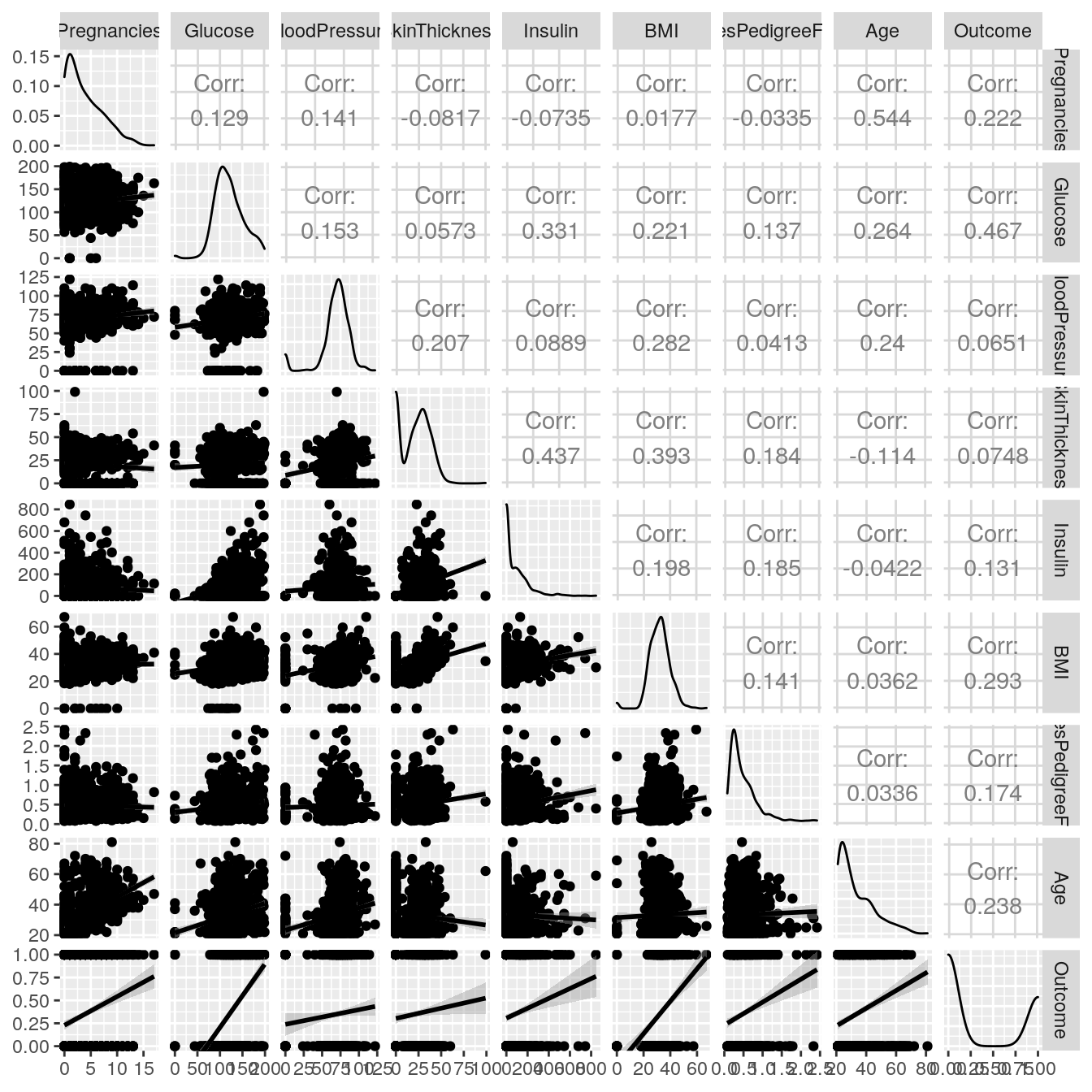
The correlations between explanatory variables do not seem too strong. Hence the model is not likely to suffer from multicollinearity. All explanatory variable are correlated with the Outcome. At first sight, glucose rate is the most important factor to detect the outcome.
5.3 Logistic regression with R
After variable exploration, a first model can be fitted using the glm function. With stargazer, it is easy to get nice output in ASCII or even Latex.
# first model: all features
glm1 = glm(Outcome~.,
           DiabetesData,
           family = binomial(link="logit"))

summary(glm1)
#>
#> Call:
#> glm(formula = Outcome ~ ., family = binomial(link = "logit"),
#>     data = DiabetesData)
#>
#> Deviance Residuals:
#>    Min      1Q  Median      3Q     Max
#> -2.557  -0.727  -0.416   0.727   2.930
#>
#> Coefficients:
#>                           Estimate Std. Error z value Pr(>|z|)
#> (Intercept)              -8.404696   0.716636  -11.73  < 2e-16 ***
#> Pregnancies               0.123182   0.032078    3.84  0.00012 ***
#> Glucose                   0.035164   0.003709    9.48  < 2e-16 ***
#> BloodPressure            -0.013296   0.005234   -2.54  0.01107 *
#> SkinThickness             0.000619   0.006899    0.09  0.92852
#> Insulin                  -0.001192   0.000901   -1.32  0.18607
#> BMI                       0.089701   0.015088    5.95  2.8e-09 ***
#> DiabetesPedigreeFunction  0.945180   0.299147    3.16  0.00158 **
#> Age                       0.014869   0.009335    1.59  0.11119
#> ---
#> Signif. codes:  0 '***' 0.001 '**' 0.01 '*' 0.05 '.' 0.1 ' ' 1
#>
#> (Dispersion parameter for binomial family taken to be 1)
#>
#>     Null deviance: 993.48  on 767  degrees of freedom
#> Residual deviance: 723.45  on 759  degrees of freedom
#> AIC: 741.4
#>
#> Number of Fisher Scoring iterations: 5
require(stargazer)
#> Loading required package: stargazer
#>
#> Please cite as:
#>  Hlavac, Marek (2018). stargazer: Well-Formatted Regression and Summary Statistics Tables.
#>  R package version 5.2.2. https://CRAN.R-project.org/package=stargazer
stargazer(glm1,type='text')
#>
#> ====================================================
#>                              Dependent variable:
#>                          ---------------------------
#>                                    Outcome
#> ----------------------------------------------------
#> Pregnancies                       0.123***
#>                                    (0.032)
#>
#> Glucose                           0.035***
#>                                    (0.004)
#>
#> BloodPressure                     -0.013**
#>                                    (0.005)
#>
#> SkinThickness                       0.001
#>                                    (0.007)
#>
#> Insulin                            -0.001
#>                                    (0.001)
#>
#> BMI                               0.090***
#>                                    (0.015)
#>
#> DiabetesPedigreeFunction          0.945***
#>                                    (0.299)
#>
#> Age                                 0.015
#>                                    (0.009)
#>
#> Constant                          -8.400***
#>                                    (0.717)
#>
#> ----------------------------------------------------
#> Observations                         768
#> Log Likelihood                    -362.000
#> Akaike Inf. Crit.                  741.000
#> ====================================================
#> Note:                    *p<0.1; **p<0.05; ***p<0.01
The overall model is significant. As expected the glucose rate has the lowest p-value of all the variables. However, Age, Insulin and Skin Thickness are not good predictors of Diabetes.
5.4 A second model
Since some variables are not significant, removing them is a good way to improve model robustness. In the second model, SkinThickness, Insulin, and Age are removed.
# second model: selected features
glm2 = glm(Outcome~.,
         data = DiabetesData[,c(1:3,6:7,9), with=F],
         family = binomial(link="logit"))

summary(glm2)
#>
#> Call:
#> glm(formula = Outcome ~ ., family = binomial(link = "logit"),
#>     data = DiabetesData[, c(1:3, 6:7, 9), with = F])
#>
#> Deviance Residuals:
#>    Min      1Q  Median      3Q     Max
#> -2.793  -0.736  -0.419   0.725   2.955
#>
#> Coefficients:
#>                          Estimate Std. Error z value Pr(>|z|)
#> (Intercept)              -7.95495    0.67582  -11.77  < 2e-16 ***
#> Pregnancies               0.15349    0.02784    5.51  3.5e-08 ***
#> Glucose                   0.03466    0.00339   10.21  < 2e-16 ***
#> BloodPressure            -0.01201    0.00503   -2.39    0.017 *
#> BMI                       0.08483    0.01412    6.01  1.9e-09 ***
#> DiabetesPedigreeFunction  0.91063    0.29403    3.10    0.002 **
#> ---
#> Signif. codes:  0 '***' 0.001 '**' 0.01 '*' 0.05 '.' 0.1 ' ' 1
#>
#> (Dispersion parameter for binomial family taken to be 1)
#>
#>     Null deviance: 993.48  on 767  degrees of freedom
#> Residual deviance: 728.56  on 762  degrees of freedom
#> AIC: 740.6
#>
#> Number of Fisher Scoring iterations: 5
5.5 Classification rate and confusion matrix
Now that we have our model, let’s access its performance.
# Correctly classified observations
mean((glm2$fitted.values>0.5)==DiabetesData$Outcome)
#> [1] 0.775
Around 77.4% of all observations are correctly classified. Due to class imbalance, we need to go further with a confusion matrix.
###Confusion matrix count
RP=sum((glm2$fitted.values>=0.5)==DiabetesData$Outcome & DiabetesData$Outcome==1)
FP=sum((glm2$fitted.values>=0.5)!=DiabetesData$Outcome & DiabetesData$Outcome==0)
RN=sum((glm2$fitted.values>=0.5)==DiabetesData$Outcome & DiabetesData$Outcome==0)
FN=sum((glm2$fitted.values>=0.5)!=DiabetesData$Outcome & DiabetesData$Outcome==1)
confMat<-matrix(c(RP,FP,FN,RN),ncol = 2)
colnames(confMat)<-c("Pred Diabetes",'Pred no diabetes')
rownames(confMat)<-c("Real Diabetes",'Real no diabetes')
confMat
#>                  Pred Diabetes Pred no diabetes
#> Real Diabetes              154              114
#> Real no diabetes            59              441
The model is good to detect people who do not have diabetes. However, its performance on ill people is not great (only 154 out of 268 have been correctly classified).
You can also get the percentage of Real/False Positive/Negative:
# Confusion matrix proportion
RPR=RP/sum(DiabetesData$Outcome==1)*100
FNR=FN/sum(DiabetesData$Outcome==1)*100
FPR=FP/sum(DiabetesData$Outcome==0)*100
RNR=RN/sum(DiabetesData$Outcome==0)*100
confMat<-matrix(c(RPR,FPR,FNR,RNR),ncol = 2)
colnames(confMat)<-c("Pred Diabetes",'Pred no diabetes')
rownames(confMat)<-c("Real Diabetes",'Real no diabetes')
confMat
#>                  Pred Diabetes Pred no diabetes
#> Real Diabetes             57.5             42.5
#> Real no diabetes          11.8             88.2
And here is the matrix, 57.5% of people with diabetes are correctly classified. A way to improve the false negative rate would lower the detection threshold. However, as a consequence, the false positive rate would increase.
5.6 Plots and decision boundaries
The two strongest predictors of the outcome are Glucose rate and BMI. High glucose rate and high BMI are strong indicators of Diabetes.
# Plot and decision boundaries
DiabetesData$Predicted <- glm2$fitted.values

ggplot(DiabetesData, aes(x = BMI, y = Glucose, color = Predicted > 0.5)) +
    geom_point(size=2, alpha=0.5)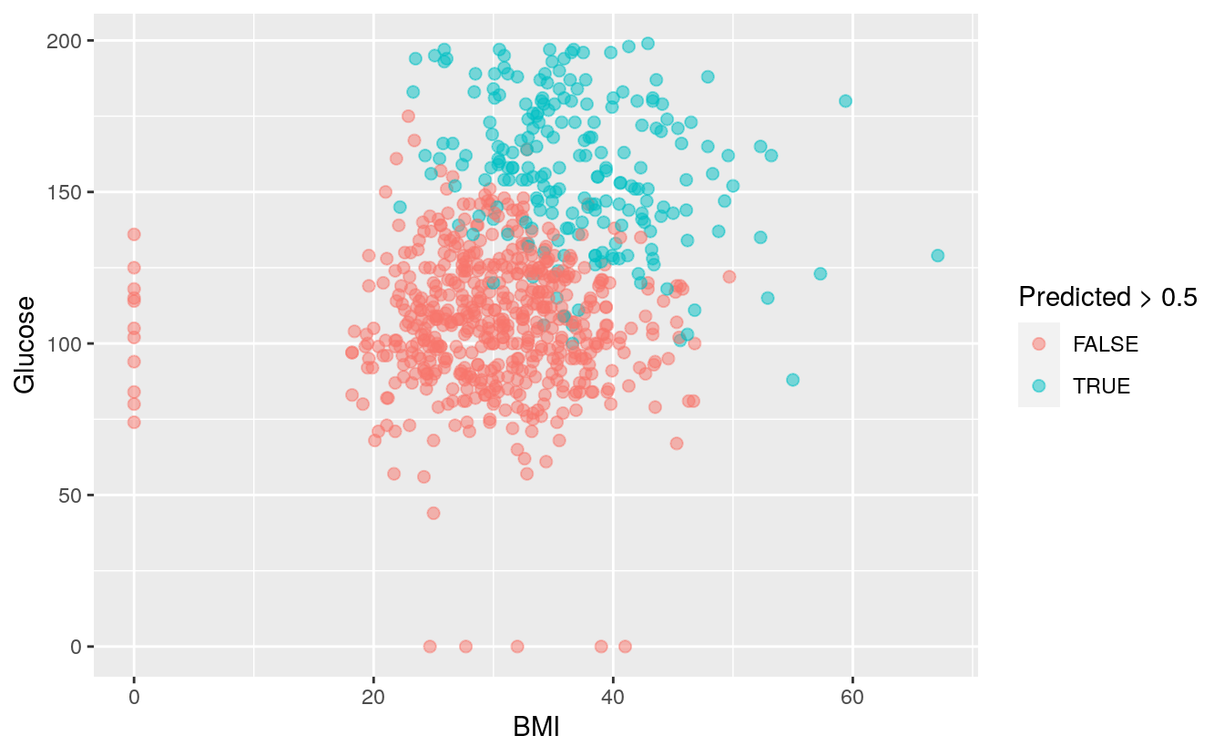
ggplot(DiabetesData, aes(x=BMI, y = Glucose, color=Outcome == (Predicted > 0.5))) +
    geom_point(size=2, alpha=0.5)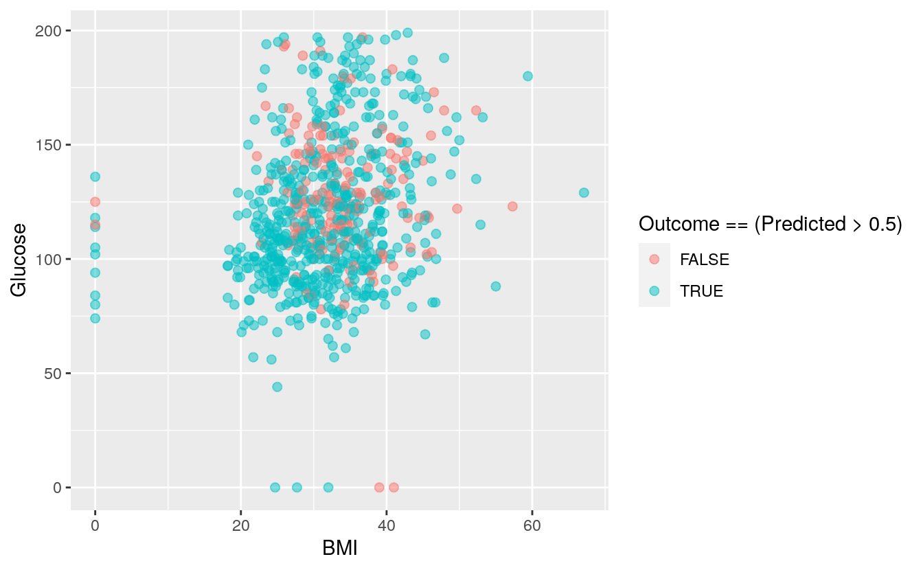
We can also plot both BMI and glucose against the outcomes, the other variables are taken at their mean level.
range(DiabetesData$BMI)
#> [1]  0.0 67.1
# BMI vs predicted
BMI_plot = data.frame(BMI = ((min(DiabetesData$BMI-2)*100):
                               (max(DiabetesData$BMI+2)*100))/100,
                    Glucose = mean(DiabetesData$Glucose),
                    Pregnancies = mean(DiabetesData$Pregnancies),
                    BloodPressure = mean(DiabetesData$BloodPressure),
                    DiabetesPedigreeFunction = mean(DiabetesData$DiabetesPedigreeFunction))

BMI_plot$Predicted = predict(glm2, newdata = BMI_plot, type = 'response')
ggplot(BMI_plot, aes(x = BMI, y = Predicted)) +
    geom_line()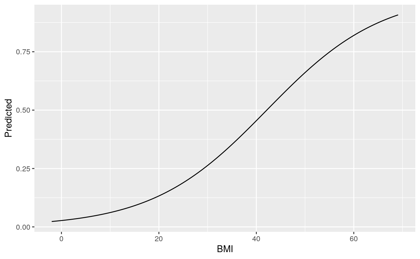
range(BMI_plot$BMI)
#> [1] -2.0 69.1
range(DiabetesData$Glucose)
#> [1]   0 199
# Glucose vs predicted
Glucose_plot=data.frame(Glucose =
                        ((min(DiabetesData$Glucose-2)*100):
                             (max(DiabetesData$Glucose+2)*100))/100,
                    BMI=mean(DiabetesData$BMI),
                    Pregnancies=mean(DiabetesData$Pregnancies),
                    BloodPressure=mean(DiabetesData$BloodPressure),
                    DiabetesPedigreeFunction=mean(DiabetesData$DiabetesPedigreeFunction))

Glucose_plot$Predicted = predict(glm2, newdata = Glucose_plot, type = 'response')
ggplot(Glucose_plot, aes(x = Glucose, y = Predicted)) +
    geom_line()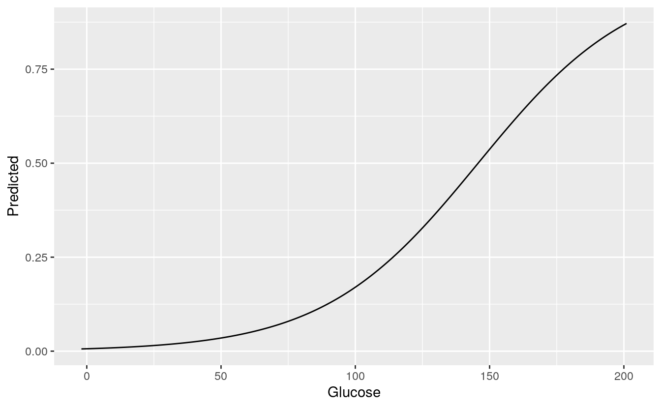
range(Glucose_plot$Glucose)
#> [1]  -2 201