3 Comparison of two PCA packages
Datasets:
decathlon2-
Algorithms:
- PCA
3.2 General methods for principal component analysis
There are two general methods to perform PCA in R :
- Spectral decomposition which examines the covariances / correlations between variables
- Singular value decomposition which examines the covariances / correlations between individuals
The function princomp() uses the spectral decomposition approach. The functions prcomp() and PCA()[FactoMineR] use the singular value decomposition (SVD).
3.2.1 prcomp() and princomp() functions
The simplified format of these 2 functions are :
prcomp(x, scale = FALSE)
princomp(x, cor = FALSE, scores = TRUE)
Arguments for prcomp():
x: a numeric matrix or data framescale: a logical value indicating whether the variables should be scaled to have unit variance before the analysis takes placeArguments for princomp():
x: a numeric matrix or data framecor: a logical value. If TRUE, the data will be centered and scaled before the analysisscores: a logical value. If TRUE, the coordinates on each principal component are calculated
3.2.2 Loading factoextra
# install.packages("factoextra")
library(factoextra)
#> Loading required package: ggplot2
#> Welcome! Want to learn more? See two factoextra-related books at https://goo.gl/ve3WBa
3.2.3 Loading the decathlon dataset
We’ll use the data sets decathlon2 [in factoextra], which has been already described at: PCA - Data format.
Briefly, it contains:
- Active individuals (rows 1 to 23) and active variables (columns 1 to 10), which are used to perform the principal component analysis
- Supplementary individuals (rows 24 to 27) and supplementary variables (columns 11 to 13), which coordinates will be predicted using the PCA information and parameters obtained with active individuals/variables.
library("factoextra")
data(decathlon2)
decathlon2.active <- decathlon2[1:23, 1:10]
head(decathlon2.active[, 1:6])
#>           X100m Long.jump Shot.put High.jump X400m X110m.hurdle
#> SEBRLE     11.0      7.58     14.8      2.07  49.8         14.7
#> CLAY       10.8      7.40     14.3      1.86  49.4         14.1
#> BERNARD    11.0      7.23     14.2      1.92  48.9         15.0
#> YURKOV     11.3      7.09     15.2      2.10  50.4         15.3
#> ZSIVOCZKY  11.1      7.30     13.5      2.01  48.6         14.2
#> McMULLEN   10.8      7.31     13.8      2.13  49.9         14.4
decathlon2.supplementary <- decathlon2[24:27, 1:10]
head(decathlon2.supplementary[, 1:6])
#>         X100m Long.jump Shot.put High.jump X400m X110m.hurdle
#> KARPOV   11.0      7.30     14.8      2.04  48.4         14.1
#> WARNERS  11.1      7.60     14.3      1.98  48.7         14.2
#> Nool     10.8      7.53     14.3      1.88  48.8         14.8
#> Drews    10.9      7.38     13.1      1.88  48.5         14.0
3.3 Compute PCA in R using prcomp()
In this section we’ll provide an easy-to-use R code to compute and visualize PCA in R using the prcomp() function and the factoextra package.
`. Load factoextra for visualization
- compute PCA
# compute PCA
res.pca <- prcomp(decathlon2.active, scale = TRUE)- Visualize eigenvalues (scree plot). Show the percentage of variances explained by each principal component.
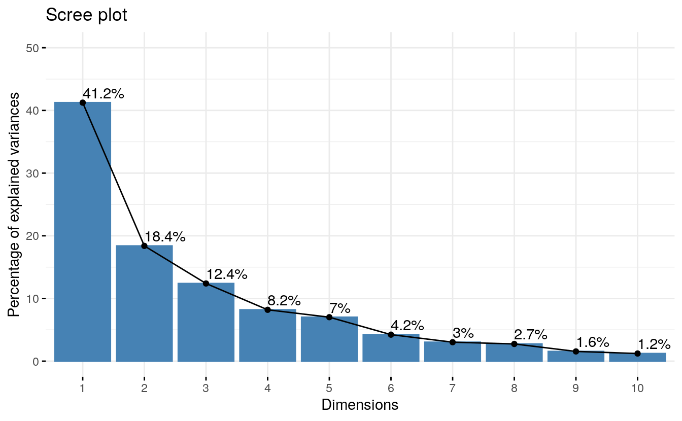
From the plot above, we might want to stop at the fifth principal component. 87% of the information (variances) contained in the data are retained by the first five principal components.
3.4 Plots: quality and contribution
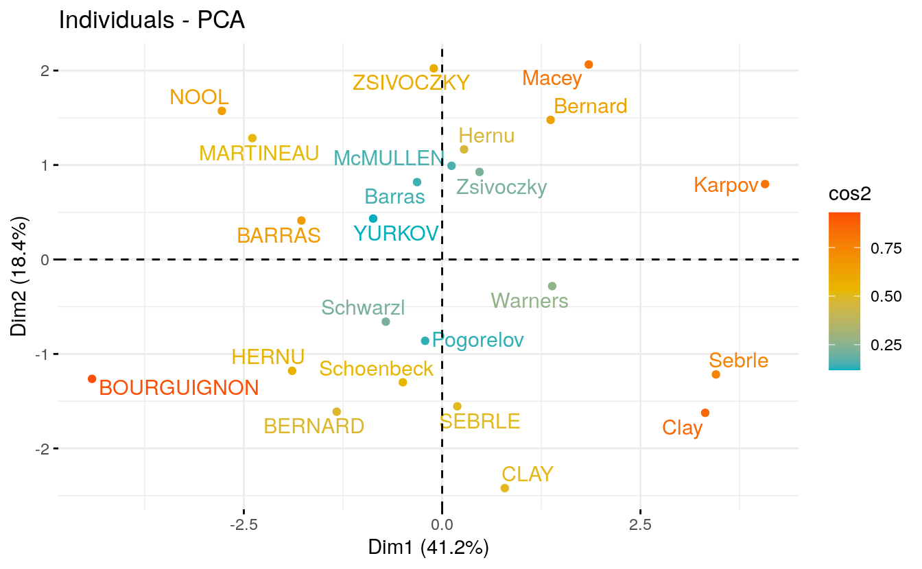
- Graph of individuals. Individuals with a similar profile are grouped together.
# Graph of individuals.
fviz_pca_ind(res.pca,
             col.ind = "cos2", # Color by the quality of representation
             gradient.cols = c("#00AFBB", "#E7B800", "#FC4E07"),
             repel = TRUE     # Avoid text overlapping
             )
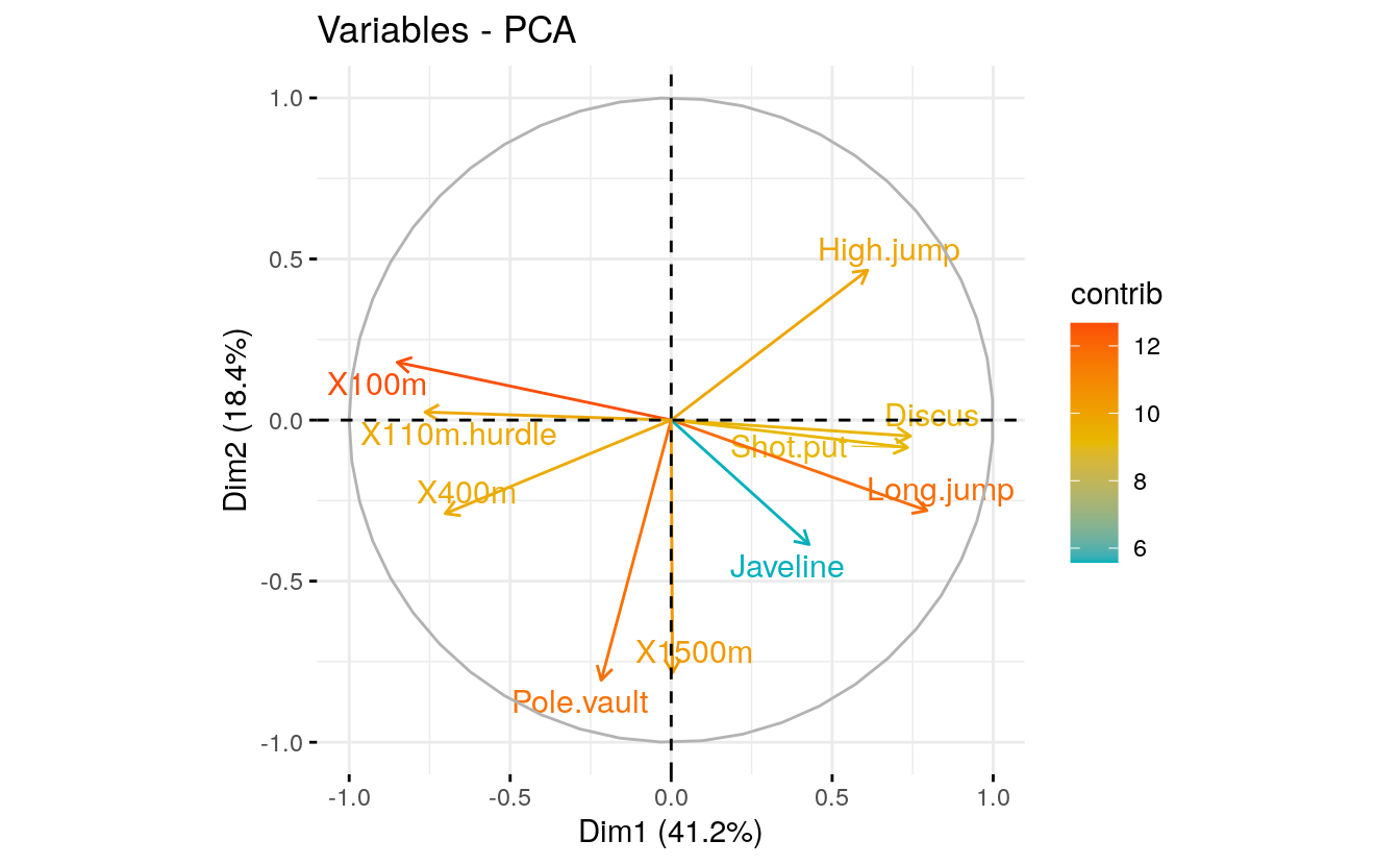
- Graph of variables. Positive correlated variables point to the same side of the plot. Negative correlated variables point to opposite sides of the graph.
# Graph of variables.
fviz_pca_var(res.pca,
             col.var = "contrib", # Color by contributions to the PC
             gradient.cols = c("#00AFBB", "#E7B800", "#FC4E07"),
             repel = TRUE     # Avoid text overlapping
             )
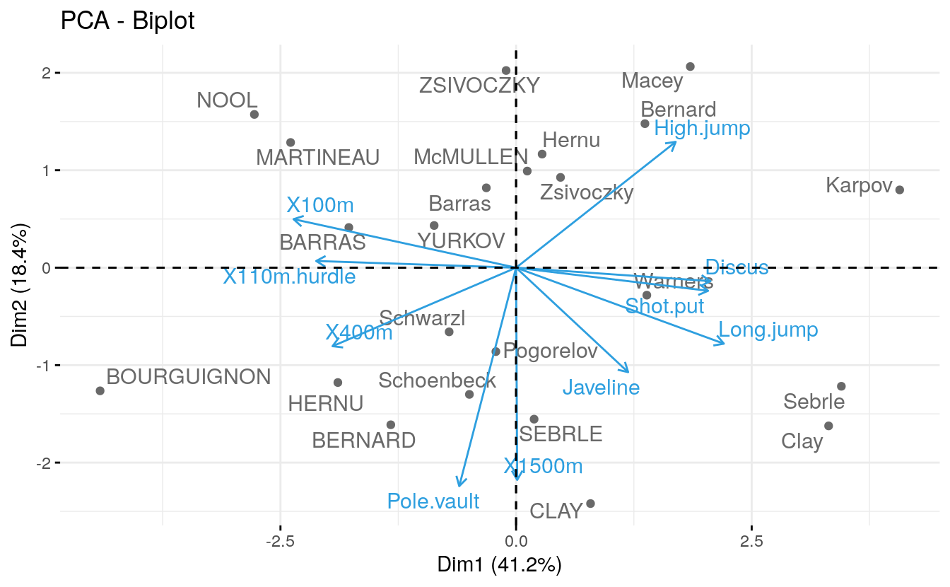
- Biplot of individuals and variables
# Biplot of individuals and variables
fviz_pca_biplot(res.pca, repel = TRUE,
                col.var = "#2E9FDF", # Variables color
                col.ind = "#696969"  # Individuals color
                )
3.5 Access to the PCA results
library(factoextra)
# Eigenvalues
eig.val <- get_eigenvalue(res.pca)
eig.val
#>        eigenvalue variance.percent cumulative.variance.percent
#> Dim.1       4.124            41.24                        41.2
#> Dim.2       1.839            18.39                        59.6
#> Dim.3       1.239            12.39                        72.0
#> Dim.4       0.819             8.19                        80.2
#> Dim.5       0.702             7.02                        87.2
#> Dim.6       0.423             4.23                        91.5
#> Dim.7       0.303             3.03                        94.5
#> Dim.8       0.274             2.74                        97.2
#> Dim.9       0.155             1.55                        98.8
#> Dim.10      0.122             1.22                       100.0

# Results for Variables
res.var <- get_pca_var(res.pca)
res.var$coord          # Coordinates
#>                 Dim.1   Dim.2   Dim.3   Dim.4  Dim.5    Dim.6    Dim.7    Dim.8
#> X100m        -0.85063  0.1794 -0.3016  0.0336 -0.194  0.03537 -0.09134 -0.10472
#> Long.jump     0.79418 -0.2809  0.1905 -0.1154  0.233 -0.03373 -0.15433 -0.39738
#> Shot.put      0.73391 -0.0854 -0.5176  0.1285 -0.249 -0.23979 -0.00989  0.02436
#> High.jump     0.61008  0.4652 -0.3301  0.1446  0.403 -0.28464  0.02816  0.08441
#> X400m        -0.70160 -0.2902 -0.2835  0.4308  0.104 -0.04929  0.28611 -0.23355
#> X110m.hurdle -0.76413  0.0247 -0.4489 -0.0169  0.224  0.00263 -0.37007 -0.00834
#> Discus        0.74321 -0.0497 -0.1765  0.3950 -0.408  0.19854 -0.14273 -0.03956
#> Pole.vault   -0.21727 -0.8075 -0.0941 -0.3390 -0.222 -0.32746 -0.01039  0.03291
#> Javeline      0.42823 -0.3861 -0.6041 -0.3317  0.198  0.36210  0.13356  0.05284
#> X1500m        0.00428 -0.7845  0.2195  0.4480  0.263  0.04205 -0.11137  0.19447
#>                Dim.9   Dim.10
#> X100m        -0.3031  0.04442
#> Long.jump    -0.0516  0.02972
#> Shot.put      0.0478  0.21745
#> High.jump    -0.1121 -0.13357
#> X400m         0.0822 -0.03417
#> X110m.hurdle  0.1618 -0.01563
#> Discus        0.0134 -0.17259
#> Pole.vault   -0.0258 -0.13721
#> Javeline     -0.0405 -0.00385
#> X1500m       -0.1022  0.06283
res.var$contrib        # Contributions to the PCs
#>                 Dim.1   Dim.2  Dim.3   Dim.4 Dim.5    Dim.6   Dim.7   Dim.8
#> X100m        1.75e+01  1.7505  7.339  0.1376  5.39  0.29592  2.7571  3.9952
#> Long.jump    1.53e+01  4.2904  2.930  1.6249  7.75  0.26900  7.8716 57.5332
#> Shot.put     1.31e+01  0.3967 21.620  2.0141  8.82 13.59686  0.0323  0.2162
#> High.jump    9.02e+00 11.7716  8.793  2.5499 23.12 19.15961  0.2620  2.5957
#> X400m        1.19e+01  4.5799  6.488 22.6509  1.54  0.57451 27.0527 19.8734
#> X110m.hurdle 1.42e+01  0.0333 16.261  0.0348  7.17  0.00164 45.2616  0.0254
#> Discus       1.34e+01  0.1341  2.515 19.0413 23.76  9.32175  6.7323  0.5702
#> Pole.vault   1.14e+00 35.4619  0.714 14.0231  7.01 25.35762  0.0357  0.3947
#> Javeline     4.45e+00  8.1087 29.453 13.4296  5.58 31.00496  5.8957  1.0173
#> X1500m       4.44e-04 33.4729  3.887 24.4939  9.88  0.41813  4.0989 13.7787
#>               Dim.9  Dim.10
#> X100m        59.174  1.6176
#> Long.jump     1.715  0.7241
#> Shot.put      1.471 38.7677
#> High.jump     8.102 14.6265
#> X400m         4.349  0.9573
#> X110m.hurdle 16.858  0.2003
#> Discus        0.115 24.4217
#> Pole.vault    0.428 15.4356
#> Javeline      1.054  0.0122
#> X1500m        6.734  3.2370
res.var$cos2           # Quality of representation
#>                 Dim.1    Dim.2   Dim.3    Dim.4  Dim.5    Dim.6    Dim.7
#> X100m        7.24e-01 0.032184 0.09094 0.001127 0.0378 1.25e-03 8.34e-03
#> Long.jump    6.31e-01 0.078881 0.03631 0.013315 0.0544 1.14e-03 2.38e-02
#> Shot.put     5.39e-01 0.007294 0.26791 0.016504 0.0619 5.75e-02 9.77e-05
#> High.jump    3.72e-01 0.216424 0.10896 0.020895 0.1622 8.10e-02 7.93e-04
#> X400m        4.92e-01 0.084203 0.08039 0.185611 0.0108 2.43e-03 8.19e-02
#> X110m.hurdle 5.84e-01 0.000612 0.20150 0.000285 0.0503 6.93e-06 1.37e-01
#> Discus       5.52e-01 0.002466 0.03116 0.156032 0.1667 3.94e-02 2.04e-02
#> Pole.vault   4.72e-02 0.651977 0.00885 0.114911 0.0491 1.07e-01 1.08e-04
#> Javeline     1.83e-01 0.149080 0.36497 0.110048 0.0391 1.31e-01 1.78e-02
#> X1500m       1.83e-05 0.615409 0.04817 0.200713 0.0693 1.77e-03 1.24e-02
#>                 Dim.8    Dim.9   Dim.10
#> X100m        1.10e-02 0.091848 1.97e-03
#> Long.jump    1.58e-01 0.002661 8.83e-04
#> Shot.put     5.93e-04 0.002284 4.73e-02
#> High.jump    7.12e-03 0.012575 1.78e-02
#> X400m        5.45e-02 0.006750 1.17e-03
#> X110m.hurdle 6.96e-05 0.026166 2.44e-04
#> Discus       1.56e-03 0.000179 2.98e-02
#> Pole.vault   1.08e-03 0.000664 1.88e-02
#> Javeline     2.79e-03 0.001637 1.49e-05
#> X1500m       3.78e-02 0.010453 3.95e-03
# Results for individuals
res.ind <- get_pca_ind(res.pca)
res.ind$coord          # Coordinates
#>              Dim.1  Dim.2  Dim.3   Dim.4     Dim.5   Dim.6   Dim.7    Dim.8
#> SEBRLE       0.191 -1.554 -0.628  0.0821  1.142614 -0.4639 -0.2080  0.04346
#> CLAY         0.790 -2.420  1.357  1.2698 -0.806848  1.3042 -0.2129  0.61724
#> BERNARD     -1.329 -1.612 -0.196 -1.9209  0.082343 -0.4006 -0.4064  0.70386
#> YURKOV      -0.869  0.433 -2.474  0.6972  0.398858  0.1029 -0.3249  0.11500
#> ZSIVOCZKY   -0.106  2.023  1.305 -0.0993 -0.197024  0.8955  0.0883 -0.20234
#> McMULLEN     0.119  0.992  0.844  1.3122  1.585871  0.1866  0.4783  0.29309
#> MARTINEAU   -2.392  1.285 -0.898  0.3731 -2.243352 -0.4567 -0.2998 -0.29163
#> HERNU       -1.891 -1.178 -0.156  0.8913 -0.126741  0.4362 -0.5661 -1.52940
#> BARRAS      -1.774  0.413  0.658  0.2287 -0.233837  0.0903  0.2159  0.68258
#> NOOL        -2.777  1.573  0.607 -1.5555  1.424184  0.4972 -0.5321 -0.43339
#> BOURGUIGNON -4.414 -1.264 -0.010  0.6668  0.419152 -0.0820 -0.5983  0.56362
#> Sebrle       3.451 -1.217 -1.678 -0.8087 -0.025053 -0.0828  0.0102 -0.03059
#> Clay         3.316 -1.623 -0.618 -0.3168  0.569165  0.7772  0.2575 -0.58064
#> Karpov       4.070  0.798  1.015  0.3134 -0.797426 -0.3296 -1.3637  0.34531
#> Macey        1.848  2.064 -0.979  0.5847 -0.000216 -0.1973 -0.2693 -0.36322
#> Warners      1.387 -0.282  2.000 -1.0196 -0.040540 -0.5567 -0.2674 -0.10947
#> Zsivoczky    0.472  0.927 -1.728 -0.1848  0.407303 -0.1138  0.0399  0.53804
#> Hernu        0.276  1.166  0.171 -0.8487 -0.689480 -0.3317  0.4431  0.24729
#> Bernard      1.367  1.478  0.831  0.7453  0.859802 -0.3281  0.3636  0.00617
#> Schwarzl    -0.710 -0.658  1.041 -0.9272 -0.288757 -0.6889  0.5657 -0.68705
#> Pogorelov   -0.214 -0.861  0.298  1.3556 -0.015053 -1.5938  0.7837 -0.03762
#> Schoenbeck  -0.495 -1.300  0.103 -0.2493 -0.645226  0.1617  0.8575 -0.25585
#> Barras      -0.316  0.819 -0.862 -0.5894 -0.779739  1.1742  0.9451  0.36555
#>                Dim.9  Dim.10
#> SEBRLE      -0.65934  0.0327
#> CLAY        -0.06013 -0.3172
#> BERNARD      0.17008 -0.0991
#> YURKOV      -0.10952 -0.1197
#> ZSIVOCZKY   -0.52310 -0.3484
#> McMULLEN    -0.10562 -0.3932
#> MARTINEAU   -0.22342 -0.6164
#> HERNU        0.00618  0.5537
#> BARRAS      -0.66928  0.5309
#> NOOL        -0.11578 -0.0962
#> BOURGUIGNON  0.52581  0.0586
#> Sebrle      -0.84721  0.2197
#> Clay         0.40978 -0.6160
#> Karpov       0.19306  0.2172
#> Macey        0.36826  0.2125
#> Warners      0.18028  0.2421
#> Zsivoczky    0.58597 -0.1427
#> Hernu        0.06691 -0.2087
#> Bernard      0.27949  0.3207
#> Schwarzl    -0.00836 -0.3021
#> Pogorelov   -0.13053 -0.0370
#> Schoenbeck   0.56422  0.2968
#> Barras       0.10226  0.6119
res.ind$contrib        # Contributions to the PCs
#>               Dim.1  Dim.2    Dim.3   Dim.4    Dim.5   Dim.6    Dim.7    Dim.8
#> SEBRLE       0.0385  5.712 1.39e+00  0.0357 8.09e+00  2.2126  0.62143 2.99e-02
#> CLAY         0.6581 13.854 6.46e+00  8.5557 4.03e+00 17.4880  0.65141 6.04e+00
#> BERNARD      1.8627  6.144 1.35e-01 19.5783 4.20e-02  1.6502  2.37365 7.85e+00
#> YURKOV       0.7969  0.443 2.15e+01  2.5794 9.86e-01  0.1088  1.51656 2.09e-01
#> ZSIVOCZKY    0.0118  9.682 5.97e+00  0.0523 2.41e-01  8.2456  0.11192 6.49e-01
#> McMULLEN     0.0148  2.325 2.50e+00  9.1353 1.56e+01  0.3579  3.28702 1.36e+00
#> MARTINEAU    6.0337  3.904 2.83e+00  0.7386 3.12e+01  2.1441  1.29111 1.35e+00
#> HERNU        3.7700  3.284 8.58e-02  4.2151 9.96e-02  1.9566  4.60485 3.71e+01
#> BARRAS       3.3194  0.402 1.52e+00  0.2776 3.39e-01  0.0838  0.67004 7.38e+00
#> NOOL         8.1299  5.849 1.29e+00 12.8376 1.26e+01  2.5413  4.06767 2.98e+00
#> BOURGUIGNON 20.5373  3.776 3.53e-04  2.3588 1.09e+00  0.0691  5.14425 5.03e+00
#> Sebrle      12.5584  3.502 9.88e+00  3.4701 3.89e-03  0.0705  0.00148 1.48e-02
#> Clay        11.5936  6.232 1.34e+00  0.5325 2.01e+00  6.2097  0.95282 5.34e+00
#> Karpov      17.4661  1.507 3.61e+00  0.5210 3.94e+00  1.1168 26.72016 1.89e+00
#> Macey        3.6021 10.073 3.36e+00  1.8139 2.89e-07  0.4001  1.04191 2.09e+00
#> Warners      2.0291  0.188 1.40e+01  5.5159 1.02e-02  3.1867  1.02738 1.90e-01
#> Zsivoczky    0.2344  2.031 1.05e+01  0.1813 1.03e+00  0.1332  0.02289 4.59e+00
#> Hernu        0.0805  3.214 1.02e-01  3.8217 2.95e+00  1.1311  2.82103 9.69e-01
#> Bernard      1.9708  5.166 2.43e+00  2.9474 4.58e+00  1.1066  1.89945 6.02e-04
#> Schwarzl     0.5318  1.025 3.80e+00  4.5612 5.17e-01  4.8796  4.59812 7.48e+00
#> Pogorelov    0.0484  1.753 3.11e-01  9.7503 1.40e-03 26.1167  8.82532 2.24e-02
#> Schoenbeck   0.2586  3.997 3.72e-02  0.3297 2.58e+00  0.2689 10.56627 1.04e+00
#> Barras       0.1052  1.588 2.61e+00  1.8430 3.77e+00 14.1743 12.83542 2.12e+00
#>                Dim.9  Dim.10
#> SEBRLE      12.17748  0.0382
#> CLAY         0.10126  3.5857
#> BERNARD      0.81032  0.3499
#> YURKOV       0.33601  0.5107
#> ZSIVOCZKY    7.66492  4.3274
#> McMULLEN     0.31250  5.5105
#> MARTINEAU    1.39820 13.5440
#> HERNU        0.00107 10.9278
#> BARRAS      12.54733 10.0454
#> NOOL         0.37548  0.3300
#> BOURGUIGNON  7.74457  0.1222
#> Sebrle      20.10555  1.7206
#> Clay         4.70357 13.5271
#> Karpov       1.04399  1.6819
#> Macey        3.79877  1.6096
#> Warners      0.91042  2.0890
#> Zsivoczky    9.61785  0.7261
#> Hernu        0.12540  1.5523
#> Bernard      2.18807  3.6657
#> Schwarzl     0.00196  3.2536
#> Pogorelov    0.47727  0.0487
#> Schoenbeck   8.91730  3.1402
#> Barras       0.29289 13.3453
res.ind$cos2           # Quality of representation
#>               Dim.1  Dim.2    Dim.3   Dim.4    Dim.5    Dim.6    Dim.7    Dim.8
#> SEBRLE      0.00753 0.4975 8.13e-02 0.00139 2.69e-01 0.044324 8.91e-03 3.89e-04
#> CLAY        0.04870 0.4570 1.44e-01 0.12579 5.08e-02 0.132691 3.54e-03 2.97e-02
#> BERNARD     0.19720 0.2900 4.29e-03 0.41182 7.57e-04 0.017913 1.84e-02 5.53e-02
#> YURKOV      0.09611 0.0238 7.78e-01 0.06181 2.02e-02 0.001345 1.34e-02 1.68e-03
#> ZSIVOCZKY   0.00157 0.5764 2.40e-01 0.00139 5.47e-03 0.112918 1.10e-03 5.76e-03
#> McMULLEN    0.00218 0.1522 1.10e-01 0.26649 3.89e-01 0.005388 3.54e-02 1.33e-02
#> MARTINEAU   0.40401 0.1165 5.69e-02 0.00983 3.55e-01 0.014721 6.34e-03 6.00e-03
#> HERNU       0.39928 0.1551 2.73e-03 0.08870 1.79e-03 0.021248 3.58e-02 2.61e-01
#> BARRAS      0.61624 0.0333 8.48e-02 0.01024 1.07e-02 0.001594 9.13e-03 9.12e-02
#> NOOL        0.48987 0.1571 2.34e-02 0.15369 1.29e-01 0.015701 1.80e-02 1.19e-02
#> BOURGUIGNON 0.85970 0.0705 4.45e-06 0.01962 7.75e-03 0.000297 1.58e-02 1.40e-02
#> Sebrle      0.67538 0.0840 1.60e-01 0.03708 3.56e-05 0.000389 5.85e-06 5.30e-05
#> Clay        0.68759 0.1648 2.39e-02 0.00627 2.03e-02 0.037763 4.15e-03 2.11e-02
#> Karpov      0.78367 0.0301 4.87e-02 0.00464 3.01e-02 0.005138 8.80e-02 5.64e-03
#> Macey       0.36344 0.4531 1.02e-01 0.03636 4.95e-09 0.004140 7.71e-03 1.40e-02
#> Warners     0.25565 0.0106 5.31e-01 0.13808 2.18e-04 0.041169 9.50e-03 1.59e-03
#> Zsivoczky   0.04505 0.1740 6.05e-01 0.00692 3.36e-02 0.002625 3.23e-04 5.87e-02
#> Hernu       0.02482 0.4418 9.46e-03 0.23420 1.55e-01 0.035771 6.38e-02 1.99e-02
#> Bernard     0.28935 0.3381 1.07e-01 0.08598 1.14e-01 0.016659 2.05e-02 5.88e-06
#> Schwarzl    0.11672 0.1003 2.51e-01 0.19889 1.93e-02 0.109806 7.40e-02 1.09e-01
#> Pogorelov   0.00780 0.1259 1.50e-02 0.31210 3.85e-05 0.431416 1.04e-01 2.40e-04
#> Schoenbeck  0.06707 0.4620 2.90e-03 0.01699 1.14e-01 0.007150 2.01e-01 1.79e-02
#> Barras      0.01897 0.1277 1.41e-01 0.06604 1.16e-01 0.262130 1.70e-01 2.54e-02
#>                Dim.9   Dim.10
#> SEBRLE      8.95e-02 0.000221
#> CLAY        2.82e-04 0.007847
#> BERNARD     3.23e-03 0.001096
#> YURKOV      1.53e-03 0.001822
#> ZSIVOCZKY   3.85e-02 0.017092
#> McMULLEN    1.73e-03 0.023927
#> MARTINEAU   3.52e-03 0.026821
#> HERNU       4.27e-06 0.034229
#> BARRAS      8.77e-02 0.055153
#> NOOL        8.51e-04 0.000588
#> BOURGUIGNON 1.22e-02 0.000151
#> Sebrle      4.07e-02 0.002737
#> Clay        1.05e-02 0.023726
#> Karpov      1.76e-03 0.002232
#> Macey       1.44e-02 0.004803
#> Warners     4.32e-03 0.007784
#> Zsivoczky   6.96e-02 0.004127
#> Hernu       1.46e-03 0.014160
#> Bernard     1.21e-02 0.015917
#> Schwarzl    1.62e-05 0.021117
#> Pogorelov   2.89e-03 0.000232
#> Schoenbeck  8.70e-02 0.024083
#> Barras      1.99e-03 0.071184
3.6 Predict using PCA
In this section, we’ll show how to predict the coordinates of supplementary individuals and variables using only the information provided by the previously performed PCA.
- Data: rows 24 to 27 and columns 1 to to 10 [in decathlon2 data sets]. The new data must contain columns (variables) with the same names and in the same order as the active data used to compute PCA.
# Data for the supplementary individuals
ind.sup <- decathlon2[24:27, 1:10]
ind.sup[, 1:6]
#>         X100m Long.jump Shot.put High.jump X400m X110m.hurdle
#> KARPOV   11.0      7.30     14.8      2.04  48.4         14.1
#> WARNERS  11.1      7.60     14.3      1.98  48.7         14.2
#> Nool     10.8      7.53     14.3      1.88  48.8         14.8
#> Drews 10.9 7.38 13.1 1.88 48.5 14.0- Predict the coordinates of new individuals data. Use the R base function predict():
ind.sup.coord <- predict(res.pca, newdata = ind.sup)
ind.sup.coord[, 1:4]
#>            PC1    PC2   PC3    PC4
#> KARPOV   0.777 -0.762 1.597  1.686
#> WARNERS -0.378  0.119 1.701 -0.691
#> Nool    -0.547 -1.934 0.472 -2.228
#> Drews -1.085 -0.017 2.982 -1.501- Graph of individuals including the supplementary individuals:
# Plot of active individuals
p <- fviz_pca_ind(res.pca, repel = TRUE)
# Add supplementary individuals
fviz_add(p, ind.sup.coord, color ="blue")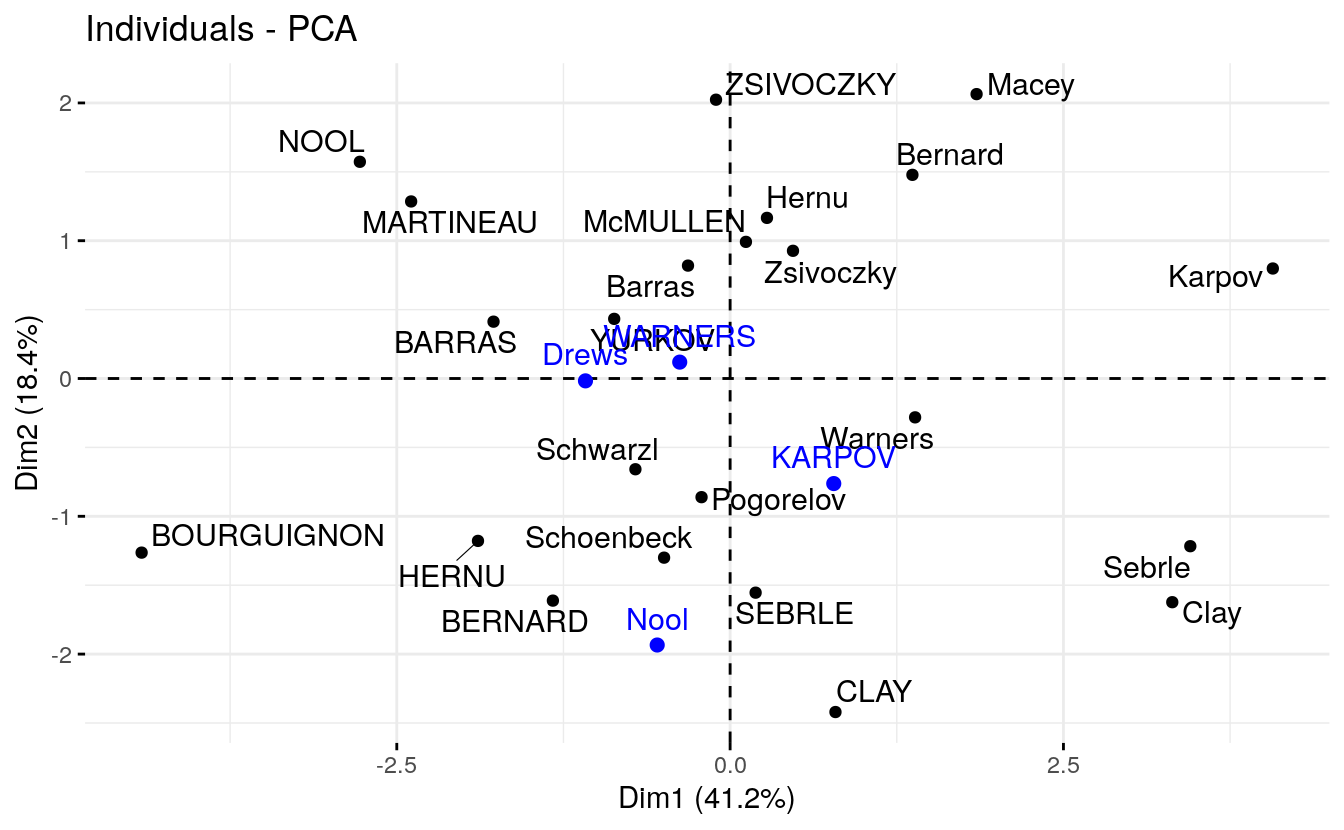
The predicted coordinates of individuals can be manually calculated as follow:
- Center and scale the new individuals data using the center and the scale of the PCA
- Calculate the predicted coordinates by multiplying the scaled values with the eigenvectors (loadings) of the principal components. The R code below can be used :
# Centering and scaling the supplementary individuals
ind.scaled <- scale(ind.sup,
                    center = res.pca$center,
                    scale = res.pca$scale)
# Coordinates of the individividuals
coord_func <- function(ind, loadings){
  r <- loadings*ind
  apply(r, 2, sum)
}
pca.loadings <- res.pca$rotation
ind.sup.coord <- t(apply(ind.scaled, 1, coord_func, pca.loadings ))
ind.sup.coord[, 1:4]
#>            PC1    PC2   PC3    PC4
#> KARPOV   0.777 -0.762 1.597  1.686
#> WARNERS -0.378  0.119 1.701 -0.691
#> Nool    -0.547 -1.934 0.472 -2.228
#> Drews   -1.085 -0.017 2.982 -1.501
3.7 Supplementary variables
3.7.1 Qualitative / categorical variables
The data sets decathlon2 contain a supplementary qualitative variable at columns 13 corresponding to the type of competitions.
Qualitative / categorical variables can be used to color individuals by groups. The grouping variable should be of same length as the number of active individuals (here 23).
groups <- as.factor(decathlon2$Competition[1:23])
fviz_pca_ind(res.pca,
             col.ind = groups, # color by groups
             palette = c("#00AFBB",  "#FC4E07"),
             addEllipses = TRUE, # Concentration ellipses
             ellipse.type = "confidence",
             legend.title = "Groups",
             repel = TRUE
             )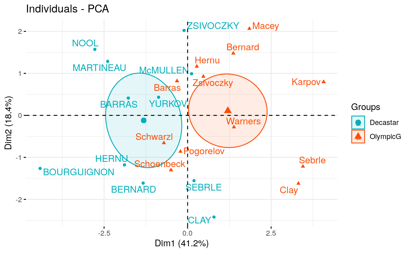
Calculate the coordinates for the levels of grouping variables. The coordinates for a given group is calculated as the mean coordinates of the individuals in the group.
library(magrittr) # for pipe %>%
library(dplyr)   # everything else
#>
#> Attaching package: 'dplyr'
#> The following objects are masked from 'package:stats':
#>
#>     filter, lag
#> The following objects are masked from 'package:base':
#>
#>     intersect, setdiff, setequal, union

# 1. Individual coordinates
res.ind <- get_pca_ind(res.pca)
# 2. Coordinate of groups
coord.groups <- res.ind$coord %>%
  as_data_frame() %>%
  select(Dim.1, Dim.2) %>%
  mutate(competition = groups) %>%
  group_by(competition) %>%
  summarise(
    Dim.1 = mean(Dim.1),
    Dim.2 = mean(Dim.2)
    )
#> Warning: `as_data_frame()` is deprecated as of tibble 2.0.0.
#> Please use `as_tibble()` instead.
#> The signature and semantics have changed, see `?as_tibble`.
#> This warning is displayed once every 8 hours.
#> Call `lifecycle::last_warnings()` to see where this warning was generated.
coord.groups
#> # A tibble: 2 x 3
#>   competition Dim.1  Dim.2
#>   <fct>       <dbl>  <dbl>
#> 1 Decastar    -1.31 -0.119
#> 2 OlympicG     1.20  0.109
3.7.2 Quantitative variables
Data: columns 11:12. Should be of same length as the number of active individuals (here 23)
quanti.sup <- decathlon2[1:23, 11:12, drop = FALSE]
head(quanti.sup)
#>           Rank Points
#> SEBRLE       1   8217
#> CLAY         2   8122
#> BERNARD      4   8067
#> YURKOV       5   8036
#> ZSIVOCZKY    7   8004
#> McMULLEN     8   7995
The coordinates of a given quantitative variable are calculated as the correlation between the quantitative variables and the principal components.
# Predict coordinates and compute cos2
quanti.coord <- cor(quanti.sup, res.pca$x)
quanti.cos2 <- quanti.coord^2
# Graph of variables including supplementary variables
p <- fviz_pca_var(res.pca)
fviz_add(p, quanti.coord, color ="blue", geom="arrow")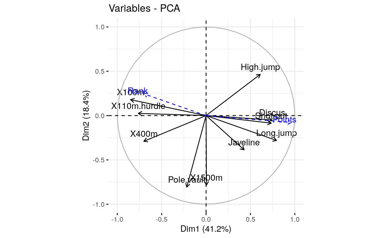
3.8 Theory behind PCA results
3.8.1 PCA results for variables
Here we’ll show how to calculate the PCA results for variables: coordinates, cos2 and contributions:
var.coord = loadings * the component standard deviations var.cos2 = var.coord^2 var.contrib. The contribution of a variable to a given principal component is (in percentage) : (var.cos2 * 100) / (total cos2 of the component)
# Helper function
#::::::::::::::::::::::::::::::::::::::::
var_coord_func <- function(loadings, comp.sdev){
  loadings*comp.sdev
}
# Compute Coordinates
#::::::::::::::::::::::::::::::::::::::::
loadings <- res.pca$rotation
sdev <- res.pca$sdev
var.coord <- t(apply(loadings, 1, var_coord_func, sdev))
head(var.coord[, 1:4])
#>                 PC1     PC2    PC3     PC4
#> X100m        -0.851  0.1794 -0.302  0.0336
#> Long.jump     0.794 -0.2809  0.191 -0.1154
#> Shot.put      0.734 -0.0854 -0.518  0.1285
#> High.jump     0.610  0.4652 -0.330  0.1446
#> X400m        -0.702 -0.2902 -0.284  0.4308
#> X110m.hurdle -0.764  0.0247 -0.449 -0.0169
# Compute Cos2
#::::::::::::::::::::::::::::::::::::::::
var.cos2 <- var.coord^2
head(var.cos2[, 1:4])
#>                PC1      PC2    PC3      PC4
#> X100m        0.724 0.032184 0.0909 0.001127
#> Long.jump    0.631 0.078881 0.0363 0.013315
#> Shot.put     0.539 0.007294 0.2679 0.016504
#> High.jump    0.372 0.216424 0.1090 0.020895
#> X400m        0.492 0.084203 0.0804 0.185611
#> X110m.hurdle 0.584 0.000612 0.2015 0.000285
# Compute contributions
#::::::::::::::::::::::::::::::::::::::::
comp.cos2 <- apply(var.cos2, 2, sum)
contrib <- function(var.cos2, comp.cos2){var.cos2*100/comp.cos2}
var.contrib <- t(apply(var.cos2,1, contrib, comp.cos2))
head(var.contrib[, 1:4])
#>                PC1     PC2   PC3     PC4
#> X100m        17.54  1.7505  7.34  0.1376
#> Long.jump    15.29  4.2904  2.93  1.6249
#> Shot.put     13.06  0.3967 21.62  2.0141
#> High.jump     9.02 11.7716  8.79  2.5499
#> X400m        11.94  4.5799  6.49 22.6509
#> X110m.hurdle 14.16  0.0333 16.26  0.0348
3.8.2 PCA results for individuals
ind.coord= res.pca$x-
Cos2 of individuals. Two steps:
- Calculate the square distance between each individual and the PCA center of gravity: d2 = [(var1_ind_i - mean_var1)/sd_var1]^2 + …+ [(var10_ind_i - mean_var10)/sd_var10]^2 + …+..
- Calculate the cos2 as ind.coord^2/d2
Contributions of individuals to the principal components: 100 * (1 / number_of_individuals)*(ind.coord^2 / comp_sdev^2). Note that the sum of all the contributions per column is 100
# Coordinates of individuals
#::::::::::::::::::::::::::::::::::
ind.coord <- res.pca$x
head(ind.coord[, 1:4])
#>              PC1    PC2    PC3     PC4
#> SEBRLE     0.191 -1.554 -0.628  0.0821
#> CLAY       0.790 -2.420  1.357  1.2698
#> BERNARD   -1.329 -1.612 -0.196 -1.9209
#> YURKOV    -0.869  0.433 -2.474  0.6972
#> ZSIVOCZKY -0.106  2.023  1.305 -0.0993
#> McMULLEN   0.119  0.992  0.844  1.3122
# Cos2 of individuals
#:::::::::::::::::::::::::::::::::
# 1. square of the distance between an individual and the
# PCA center of gravity
center <- res.pca$center
scale<- res.pca$scale

getdistance <- function(ind_row, center, scale){
  return(sum(((ind_row-center)/scale)^2))
}

d2 <- apply(decathlon2.active,1, getdistance, center, scale)
# 2. Compute the cos2. The sum of each row is 1
cos2 <- function(ind.coord, d2){return(ind.coord^2/d2)}
ind.cos2 <- apply(ind.coord, 2, cos2, d2)
head(ind.cos2[, 1:4])
#>               PC1    PC2     PC3     PC4
#> SEBRLE    0.00753 0.4975 0.08133 0.00139
#> CLAY      0.04870 0.4570 0.14363 0.12579
#> BERNARD   0.19720 0.2900 0.00429 0.41182
#> YURKOV    0.09611 0.0238 0.77823 0.06181
#> ZSIVOCZKY 0.00157 0.5764 0.23975 0.00139
#> McMULLEN  0.00218 0.1522 0.11014 0.26649
# Contributions of individuals
#:::::::::::::::::::::::::::::::
contrib <- function(ind.coord, comp.sdev, n.ind){
  100*(1/n.ind)*ind.coord^2/comp.sdev^2
}
ind.contrib <- t(apply(ind.coord, 1, contrib,
                       res.pca$sdev, nrow(ind.coord)))
head(ind.contrib[, 1:4])
#>              PC1    PC2    PC3     PC4
#> SEBRLE    0.0385  5.712  1.385  0.0357
#> CLAY      0.6581 13.854  6.460  8.5557
#> BERNARD   1.8627  6.144  0.135 19.5783
#> YURKOV    0.7969  0.443 21.476  2.5794
#> ZSIVOCZKY 0.0118  9.682  5.975  0.0523
#> McMULLEN  0.0148  2.325  2.497  9.1353