34 Comparing regression models
- Dataset:
Rates.csv - Algorithms: SLR, MLR, NN
34.1 Introduction
line 29 does not plot
Source: https://www.matthewrenze.com/workshops/practical-machine-learning-with-r/lab-3b-regression.html
library(readr)

policies <- read_csv(file.path(data_raw_dir, "Rates.csv"))
#> Parsed with column specification:
#> cols(
#>   Gender = col_character(),
#>   State = col_character(),
#>   State.Rate = col_double(),
#>   Height = col_double(),
#>   Weight = col_double(),
#>   BMI = col_double(),
#>   Age = col_double(),
#>   Rate = col_double()
#> )
policies
#> # A tibble: 1,942 x 8
#>   Gender State State.Rate Height Weight   BMI   Age   Rate
#>   <chr>  <chr>      <dbl>  <dbl>  <dbl> <dbl> <dbl>  <dbl>
#> 1 Male   MA        0.100     184   67.8  20.0    77 0.332
#> 2 Male   VA        0.142     163   89.4  33.6    82 0.869
#> 3 Male   NY        0.0908    170   81.2  28.1    31 0.01
#> 4 Male   TN        0.120     175   99.7  32.6    39 0.0215
#> 5 Male   FL        0.110     184   72.1  21.3    68 0.150
#> 6 Male   WA        0.163     166   98.4  35.7    64 0.211
#> # … with 1,936 more rows
summary(policies)
#>     Gender             State             State.Rate        Height
#>  Length:1942        Length:1942        Min.   :0.001   Min.   :150
#>  Class :character   Class :character   1st Qu.:0.110   1st Qu.:162
#>  Mode  :character   Mode  :character   Median :0.128   Median :170
#>                                        Mean   :0.138   Mean   :170
#>                                        3rd Qu.:0.144   3rd Qu.:176
#>                                        Max.   :0.318   Max.   :190
#>      Weight           BMI            Age            Rate
#>  Min.   : 44.1   Min.   :16.0   Min.   :18.0   Min.   :0.001
#>  1st Qu.: 68.6   1st Qu.:23.7   1st Qu.:34.0   1st Qu.:0.015
#>  Median : 81.3   Median :28.1   Median :51.0   Median :0.046
#>  Mean   : 81.2   Mean   :28.3   Mean   :50.8   Mean   :0.138
#>  3rd Qu.: 93.8   3rd Qu.:32.5   3rd Qu.:68.0   3rd Qu.:0.173
#>  Max.   :116.5   Max.   :46.8   Max.   :84.0   Max.   :0.999
library(RColorBrewer)
palette <- brewer.pal(9, "Reds")
# plot(
#   x = policies,
#   col = palette[cut(x = policies$Rate, breaks = 9)]
#   )
library(corrgram)
#> Registered S3 method overwritten by 'seriation':
#>   method         from
#>   reorder.hclust gclus

corrgram(policies)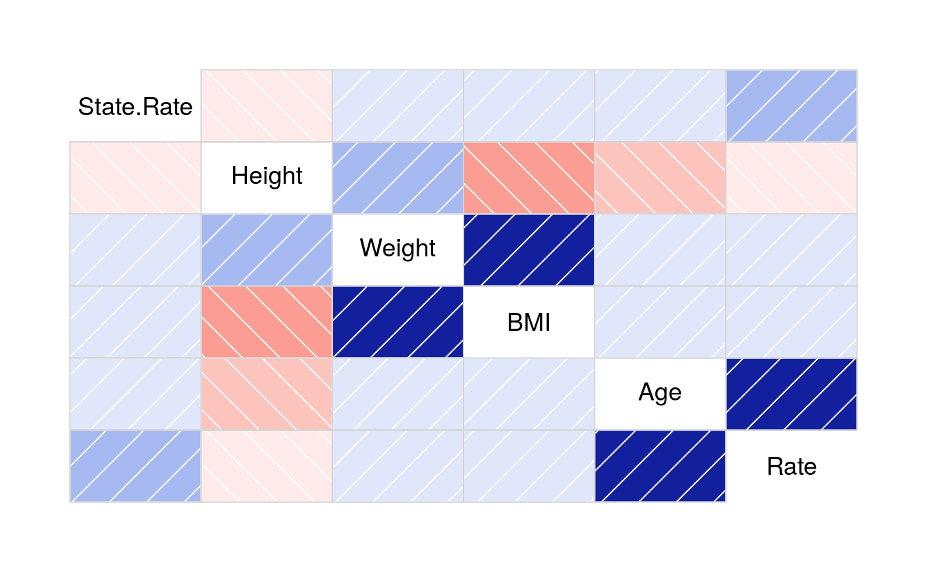
cor(policies[3:8])
#>            State.Rate  Height  Weight     BMI     Age    Rate
#> State.Rate    1.00000 -0.0165 0.00923  0.0192  0.1123  0.2269
#> Height       -0.01652  1.0000 0.23809 -0.3170 -0.1648 -0.1286
#> Weight        0.00923  0.2381 1.00000  0.8396  0.0117  0.0609
#> BMI           0.01924 -0.3170 0.83963  1.0000  0.1023  0.1405
#> Age           0.11235 -0.1648 0.01168  0.1023  1.0000  0.7801
#> Rate          0.22685 -0.1286 0.06094  0.1405  0.7801  1.0000
cor(
  x = policies$Age,
  y = policies$Rate)
#> [1] 0.78
plot(
  x = policies$Age,
  y = policies$Rate)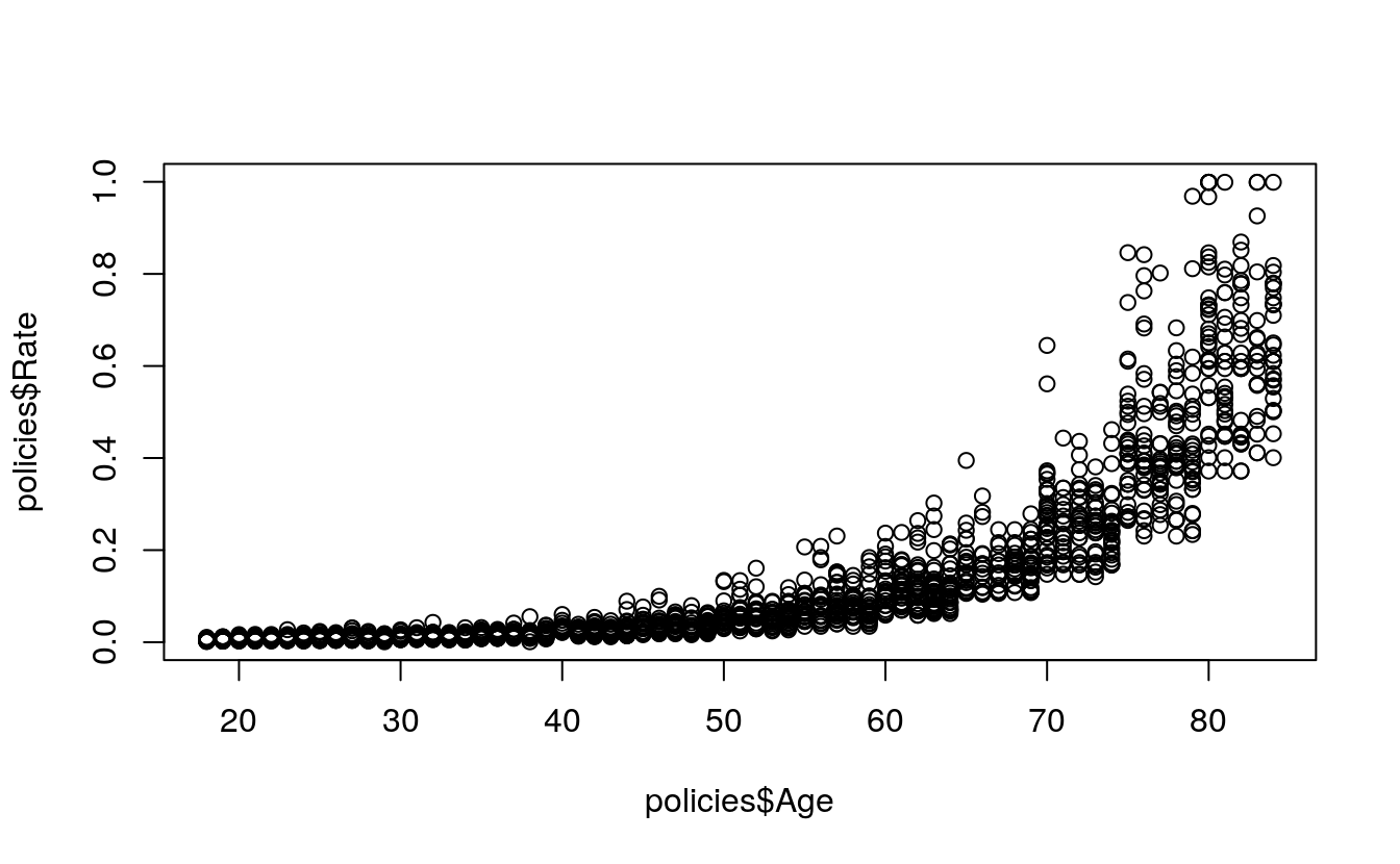
34.2 Split the Data into Test and Training Sets
set.seed(42)
library(caret)
#> Loading required package: lattice
#>
#> Attaching package: 'lattice'
#> The following object is masked from 'package:corrgram':
#>
#>     panel.fill
#> Loading required package: ggplot2

indexes <- createDataPartition(
  y = policies$Rate,
  p = 0.80,
  list = FALSE)

train <- policies[indexes, ]
#> Warning: The `i` argument of ``[`()` can't be a matrix as of tibble 3.0.0.
#> Convert to a vector.
#> This warning is displayed once every 8 hours.
#> Call `lifecycle::last_warnings()` to see where this warning was generated.
test <- policies[-indexes, ]34.3 Predict with Simple Linear Regression
simpleModel <- lm(
  formula = Rate ~ Age,
  data = train)
plot(
  x = policies$Age,
  y = policies$Rate)

lines(
  x = train$Age,
  y = simpleModel$fitted,
  col = "red",
  lwd = 3)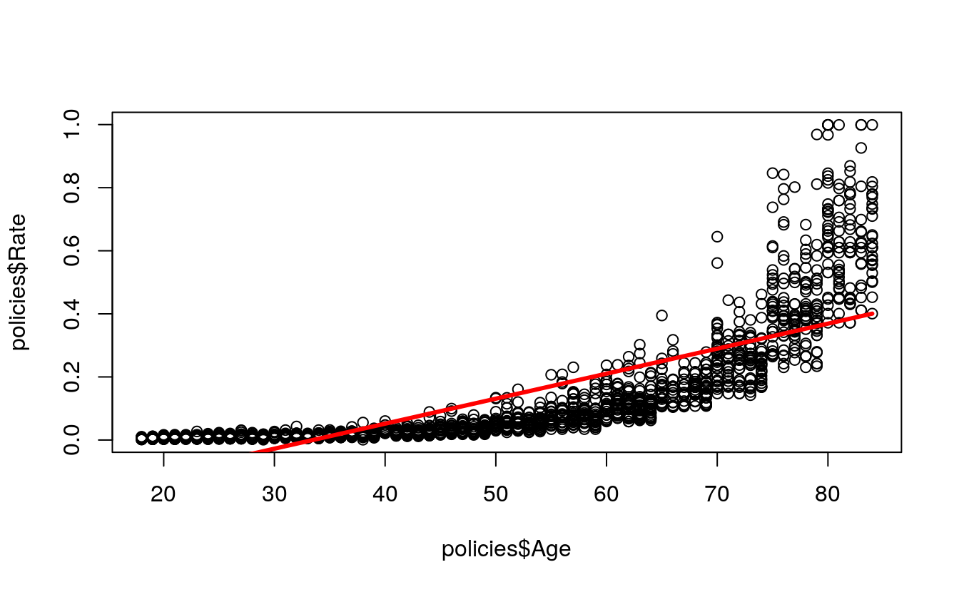
summary(simpleModel)
#>
#> Call:
#> lm(formula = Rate ~ Age, data = train)
#>
#> Residuals:
#>     Min      1Q  Median      3Q     Max
#> -0.1799 -0.0881 -0.0208  0.0617  0.6300
#>
#> Coefficients:
#>              Estimate Std. Error t value Pr(>|t|)
#> (Intercept) -0.265244   0.008780   -30.2   <2e-16 ***
#> Age          0.007928   0.000161    49.3   <2e-16 ***
#> ---
#> Signif. codes:  0 '***' 0.001 '**' 0.01 '*' 0.05 '.' 0.1 ' ' 1
#>
#> Residual standard error: 0.123 on 1553 degrees of freedom
#> Multiple R-squared:  0.61,   Adjusted R-squared:  0.609
#> F-statistic: 2.43e+03 on 1 and 1553 DF,  p-value: <2e-16
simplePredictions <- predict(
  object = simpleModel,
  newdata = test)
plot(
  x = policies$Age,
  y = policies$Rate)


points(
  x = test$Age,
  y = simplePredictions,
  col = "blue",
  pch = 4,
  lwd = 2)
34.4 Predict with Multiple Linear Regression
multipleModel <- lm(
  formula = Rate ~ Age + Gender + State.Rate + BMI,
  data = train)
summary(multipleModel)
#>
#> Call:
#> lm(formula = Rate ~ Age + Gender + State.Rate + BMI, data = train)
#>
#> Residuals:
#>     Min      1Q  Median      3Q     Max
#> -0.2255 -0.0865 -0.0292  0.0590  0.6053
#>
#> Coefficients:
#>              Estimate Std. Error t value Pr(>|t|)
#> (Intercept) -0.428141   0.018742  -22.84  < 2e-16 ***
#> Age          0.007703   0.000156   49.28  < 2e-16 ***
#> GenderMale   0.030350   0.006001    5.06  4.8e-07 ***
#> State.Rate   0.613139   0.068330    8.97  < 2e-16 ***
#> BMI          0.002634   0.000518    5.09  4.1e-07 ***
#> ---
#> Signif. codes:  0 '***' 0.001 '**' 0.01 '*' 0.05 '.' 0.1 ' ' 1
#>
#> Residual standard error: 0.118 on 1550 degrees of freedom
#> Multiple R-squared:  0.64,   Adjusted R-squared:  0.639
#> F-statistic:  688 on 4 and 1550 DF,  p-value: <2e-16
multiplePredictions <- predict(
  object = multipleModel,
  newdata = test)
plot(
  x = policies$Age,
  y = policies$Rate)

points(
  x = test$Age,
  y = multiplePredictions,
  col = "blue",
  pch = 4,
  lwd = 2)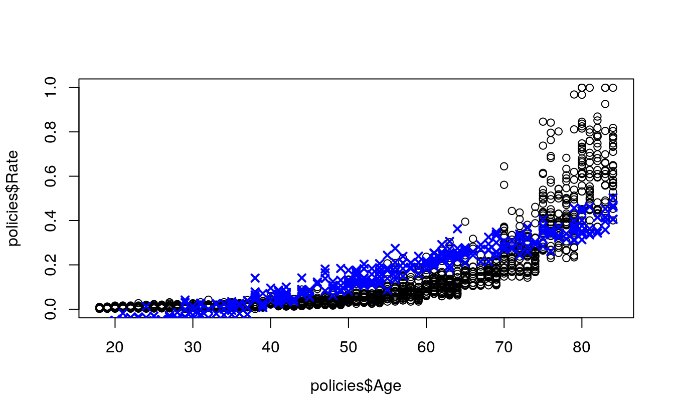
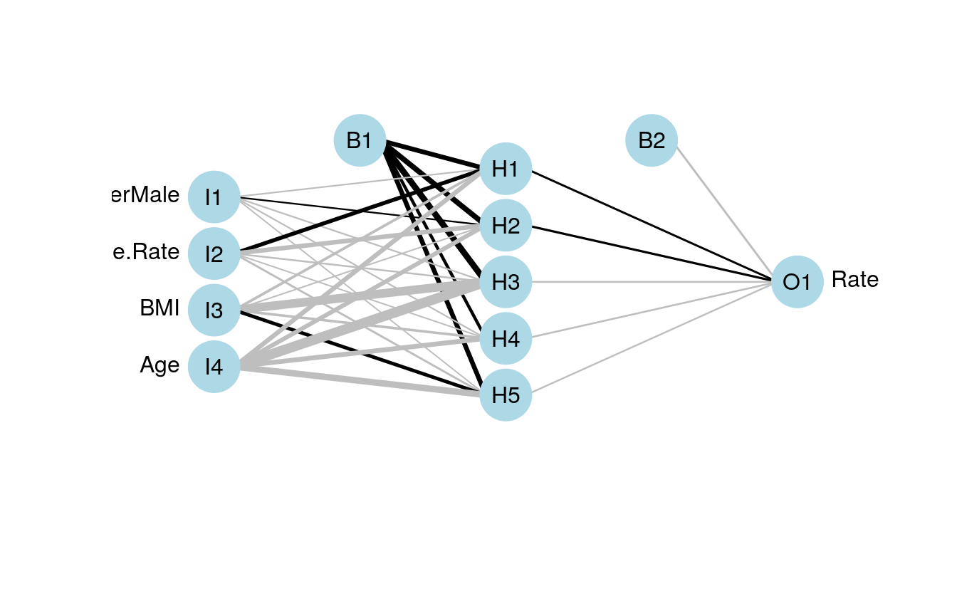
34.5 Predict with Neural Network Regression
scaledPolicies <- data.frame(
  Gender = policies$Gender,
  State.Rate = normalize(policies$State.Rate),
  BMI = normalize(policies$BMI),
  Age = normalize(policies$Age),
  Rate = normalize(policies$Rate))
scaledTrain <- scaledPolicies[indexes, ]
scaledTest <- scaledPolicies[-indexes, ]
library(nnet)

neuralRegressor <- nnet(
  formula = Rate ~ .,
  data = scaledTrain,
  linout = TRUE,
  size = 5,
  decay = 0.0001,
  maxit = 1000)
#> # weights:  31
#> initial  value 548.090539
#> iter  10 value 10.610284
#> iter  20 value 3.927378
#> iter  30 value 3.735266
#> iter  40 value 3.513899
#> iter  50 value 3.073390
#> iter  60 value 2.547202
#> iter  70 value 2.296126
#> iter  80 value 2.166120
#> iter  90 value 2.106996
#> iter 100 value 2.092654
#> iter 110 value 2.058596
#> iter 120 value 2.039404
#> iter 130 value 2.023721
#> iter 140 value 2.018777
#> iter 150 value 2.006895
#> iter 160 value 1.999130
#> iter 170 value 1.993921
#> iter 180 value 1.990505
#> iter 190 value 1.989212
#> iter 200 value 1.988818
#> iter 210 value 1.988007
#> iter 220 value 1.987710
#> iter 230 value 1.987671
#> iter 240 value 1.987599
#> iter 250 value 1.987575
#> iter 260 value 1.987553
#> iter 270 value 1.987537
#> iter 280 value 1.987528
#> final  value 1.987522
#> converged
scaledPredictions <- predict(
  object = neuralRegressor,
  newdata = scaledTest)
neuralPredictions <- denormalize(
  x = scaledPredictions,
  y = policies$Rate)
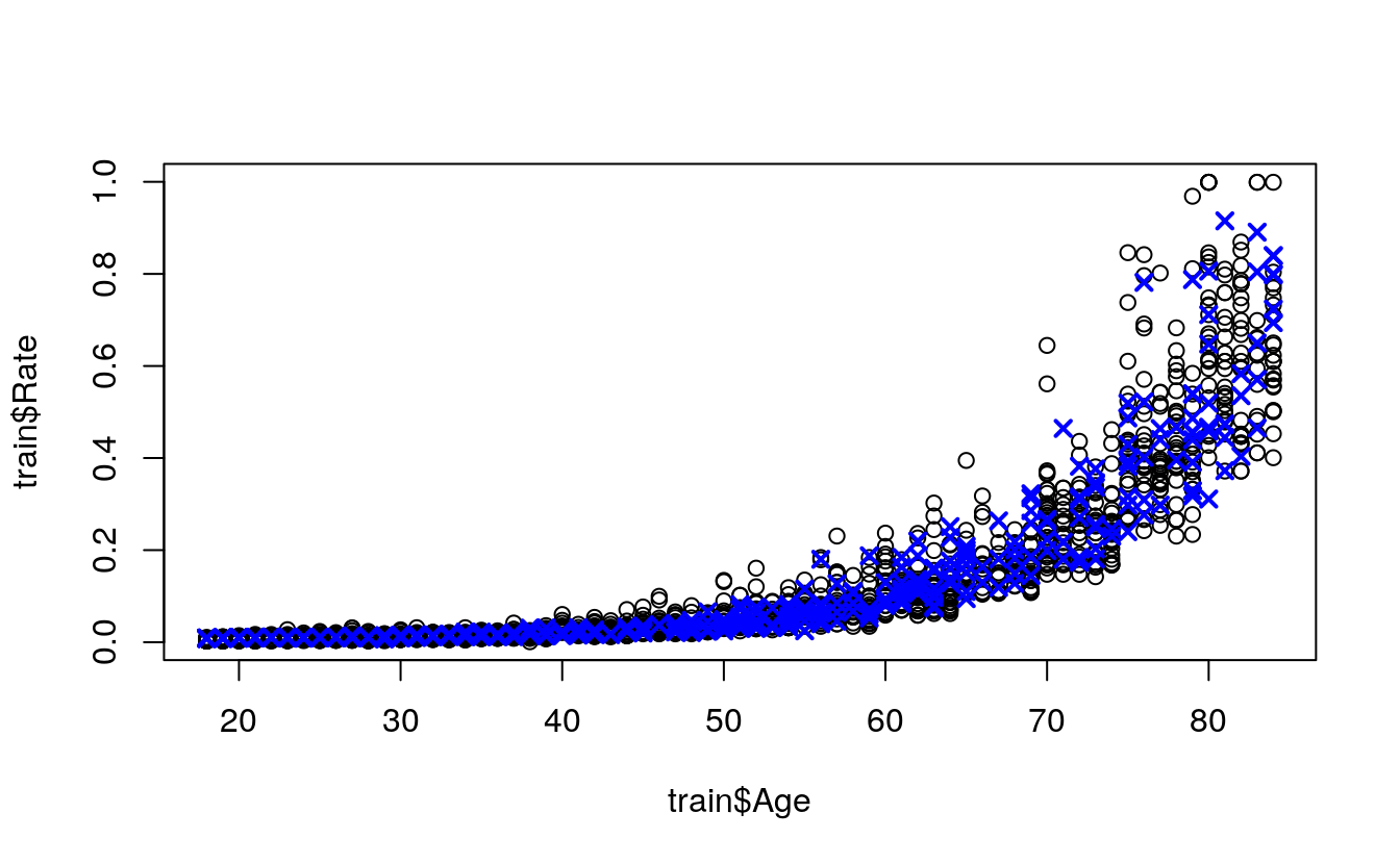
plot(
  x = train$Age,
  y = train$Rate)

points(
  x = test$Age,
  y = neuralPredictions,
  col = "blue",
  pch = 4,
  lwd = 2)