setTolerance

Set the tolerance for the solver

Set the tolerance for the solver

setTolerance(object, tol)

setTolerance(object, ...) <- value

Arguments

object	a class object
tol	tolerance
...	additional parameters
value	a value to set

Details

Sets the tolerance like this: odeSolver <- setTolerance(odeSolver, tol)

Sets the tolerance like this: setTolerance(odeSolver) <- tol

Examples

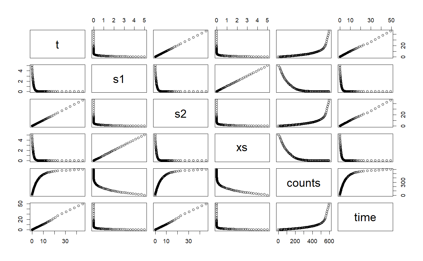
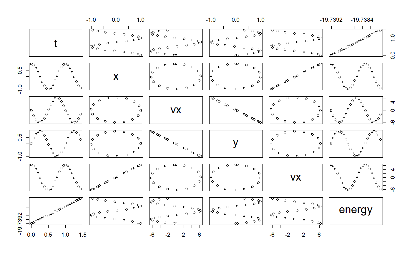
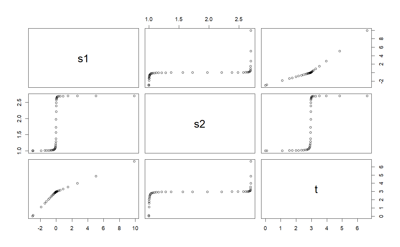
# ++++++++++++++++++++++++++++++++++++++++++++++++  example: ComparisonRK45App.R
# Compares the solution by the RK45 ODE solver versus the analytical solution
# Example file: ComparisonRK45App.R
# ODE Solver:   Runge-Kutta 45
# ODE class :   RK45
# Base class:   ODETest

importFromExamples("ODETest.R")

 ComparisonRK45App <- function(verbose = FALSE) {
     ode <- new("ODETest")                     # create an `ODETest` object
     ode_solver <- RK45(ode)                   # select the ODE solver
     ode_solver <- setStepSize(ode_solver, 1)      # set the step

     # Two ways of setting the tolerance
       # ode_solver <- setTolerance(ode_solver, 1e-8)  # set the tolerance
     setTolerance(ode_solver) <-  1e-8

     time <-  0
     rowVector <- vector("list")
     i <- 1
     while (time < 50) {
         rowVector[[i]] <- list(t  = getState(ode)[2],
                                s1 = getState(ode)[1],
                                s2 = getState(ode)[2],
                                xs = getExactSolution(ode, time),
                                counts = getRateCounts(ode),
                                time   = time
                                )
         ode_solver <- step(ode_solver)           # advance one step
         stepSize   <- getStepSize(ode_solver)
         time <- time + stepSize
         ode  <- getODE(ode_solver)                     # get updated ODE object
         i <- i + 1
     }
     return(data.table::rbindlist(rowVector))    # a data table with the results
 }
# show solution
solution <- ComparisonRK45App()                          # run the example
plot(solution)
# ++++++++++++++++++++++++++++++++++++++++++ example: KeplerDormandPrince45App.R
# Demostration of the use of ODE solver RK45 for a particle subjected to
# a inverse-law force. The difference with the example KeplerApp is we are
# seeing the effect in thex and y axis on the particle.
# The original routine used the Verlet ODE solver

importFromExamples("KeplerDormandPrince45.R")

set_solver <- function(ode_object, solver) {
    slot(ode_object, "odeSolver") <- solver
    ode_object
}

KeplerDormandPrince45App <- function(verbose = FALSE) {
    # values for the examples
    x  <- 1
    vx <- 0
    y  <- 0
    vy <- 2 * pi
    dt <- 0.01          # step size
    tol <- 1e-3         # tolerance
    particle  <- KeplerDormandPrince45()                      # use class Kepler

    # Two ways of initializing the ODE object
      # particle  <- init(particle, c(x, vx, y, vy, 0))  # enter state vector
    init(particle) <- c(x, vx, y, vy, 0)

    odeSolver <- DormandPrince45(particle)      # select the ODE solver

    # Two ways of initializing the solver
      # odeSolver <- init(odeSolver, dt)            # start the solver
    init(odeSolver) <-  dt

    # Two ways of setting the tolerance
      # odeSolver <- setTolerance(odeSolver, tol) # this works for adaptive solvers
    setTolerance(odeSolver) <- tol
    setSolver(particle) <-  odeSolver

    initialEnergy <- getEnergy(particle)        # calculate the energy
    rowVector <- vector("list")
    i <- 1
    while (getTime(particle) < 1.5) {
    rowVector[[i]] <- list(t  = getState(particle)[5],
                           x  = getState(particle)[1],
                           vx = getState(particle)[2],
                           y  = getState(particle)[3],
                           vx = getState(particle)[4],
                           energy = getEnergy(particle) )
        particle <- doStep(particle)            # advance one step
        energy   <- getEnergy(particle)         # calculate energy
        i <- i + 1
    }
    DT <- data.table::rbindlist(rowVector)
    return(DT)
}

solution <- KeplerDormandPrince45App()
plot(solution)


importFromExamples("AdaptiveStep.R")

# running function
AdaptiveStepApp <- function(verbose = FALSE) {
    ode        <- new("Impulse")
    ode_solver <- RK45(ode)

    # Two ways to initialize the solver
      # ode_solver <- init(ode_solver, 0.1)
    init(ode_solver) <- 0.1

    # two ways to set tolerance
      # ode_solver <- setTolerance(ode_solver, 1.0e-4)
    setTolerance(ode_solver) <- 1.0e-4

    i <- 1; rowVector <- vector("list")
    while (getState(ode)[1] < 12) {
        rowVector[[i]] <- list(s1 = getState(ode)[1],
                               s2 = getState(ode)[2],
                               t  = getState(ode)[3])
        ode_solver <- step(ode_solver)
        ode <- getODE(ode_solver)
        i <- i + 1
    }
    return(data.table::rbindlist(rowVector))
}

# run application
solution <- AdaptiveStepApp()
plot(solution)