2.1 Why virtual environments?

To get repeatable and reproducible results when running Python code in Rmarkdown there is nothing better than creating a Python environment.

There are several ways of running Python code. In this minimal book, we will see two of them:

• conda environments, and
• GNU Python virtualenv

Both work similarly, in the sense of providing an isolated, fresh Python environment with selected packages, without much interference of the existing Python in the operating system. Virtual environments, docker containers, and virtual machines are few of the several ways of virtualizing Python environments. This all in pursue of reproducibility: a workspace that could replicate the same results of previous analysis without the issues provoked by missing dependencies, libraries, or the operating system own environment variables.

2.2 Python virtual environment and R

Although, it is not absolutely necessary to create a virtual environment to run Rmarkdown Python notebooks, it is highly recommended because you will be able to run a selected analysis, over and over, without paying too much attention to updates or upgrades in the hosting operating system or packages updates. This means that you could freeze in time a virtual environment, without disturbing it with software updates.

This virtual environment should be able to be re-created from a text file with a minimum set of instructions, or a list of packages, or recipe, that bring a fresh Python environment, few months from now. Both, methods of creating Python virtual environments, conda and virtualenv use a text file with a recipe to do just that.

In conda there is the file environment.yml. In virtualenv, that file is named requirements.txt. But you could use any name you want. These names are just standard, and if you find them them in a repository, it mean less pain in reproducing the experiment.

2.3 conda environments

They require the installation of the Anaconda3 platform, which is pretty straight forward for all operating systems.

If you want want to create a conda virtual environment, then, you will have many ways of doing it:

conda create --name python_env python=3.7

conda create --name python_book python=3.7 pandas numpy scipy scikit-learn nltk matplotlib seaborn plotnine ipython lxml -y

conda create -n plot_env python=3.7 numpy=1.19 matplotlib=3.3 pandas=1.1 seaborn=0.11

2.4 Running Python from R

Load the reticulate library:

library(reticulate)

Load the Python environment:

use_condaenv("r-python")

Environments available and current settings:

py_config()

#:> python:         /home/msfz751/miniconda3/envs/r-python/bin/python
#:> libpython:      /home/msfz751/miniconda3/envs/r-python/lib/libpython3.7m.so
#:> pythonhome:     /home/msfz751/miniconda3/envs/r-python:/home/msfz751/miniconda3/envs/r-python
#:> version:        3.7.8 | packaged by conda-forge | (default, Jul 31 2020, 02:25:08)  [GCC 7.5.0]
#:> numpy:          /home/msfz751/miniconda3/envs/r-python/lib/python3.7/site-packages/numpy
#:> numpy_version:  1.19.4
#:> 
#:> python versions found: 
#:>  /home/msfz751/miniconda3/envs/r-python/bin/python
#:>  /home/msfz751/miniconda3/bin/python3
#:>  /usr/bin/python3
#:>  /usr/bin/python
#:>  /home/msfz751/miniconda3/envs/man_ccia/bin/python
#:>  /home/msfz751/miniconda3/envs/pybook/bin/python
#:>  /home/msfz751/miniconda3/envs/python_book/bin/python
#:>  /home/msfz751/miniconda3/envs/r-ptech/bin/python
#:>  /home/msfz751/miniconda3/envs/r-tensorflow/bin/python
#:>  /home/msfz751/miniconda3/envs/r-torch/bin/python
#:>  /home/msfz751/miniconda3/bin/python

Ask if Python is available to R:

reticulate::py_available()

#:> [1] TRUE

2.5 A plot demo

Once the environment is loaded, then our Python code chunks will just run:

Python

# https://github.com/bendichter/brokenaxes
import matplotlib
import matplotlib.pyplot as plt
import numpy as np
import matplotlib.pyplot as plt
from brokenaxes import brokenaxes
import numpy as np

fig = plt.figure(figsize=(5,5))
bax = brokenaxes(xlims=((1, 500), (600, 10000)),
         ylims=((1, 500), (600, 10000)),
         hspace=.15, xscale='log', yscale='log')

x = np.logspace(0.0, 4, 100)
bax.loglog(x, x, label='$y=x=10^{0}$ to $10^{4}$')
bax.legend(loc='best')
bax.grid(axis='both', which='major', ls='-')
bax.grid(axis='both', which='minor', ls='--', alpha=0.4)
bax.set_xlabel('x')
bax.set_ylabel('y')
plt.show()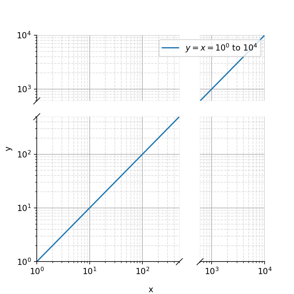

The code, you would have to type in the Rmarkdown code block, would look like this:

 ```{python}
import matplotlib
import matplotlib.pyplot as plt
import numpy as np
import matplotlib.pyplot as plt
from brokenaxes import brokenaxes
import numpy as np

fig = plt.figure(figsize=(5,5))
bax = brokenaxes(xlims=((1, 500), (600, 10000)),
     ylims=((1, 500), (600, 10000)),
         hspace=.15, xscale='log', yscale='log')

x = np.logspace(0.0, 4, 100)
bax.loglog(x, x, label='\$y=x=10\^{0}\$ to \$10\^{4}\$')

bax.legend(loc='best')
bax.grid(axis='both', which='major', ls='-')
bax.grid(axis='both', which='minor', ls='--', alpha=0.4)
bax.set_xlabel('x')
bax.set_ylabel('y')
plt.show()
```

Remember. You open a Python block in Rmarkdown with:

 ```{python}

and close it with:

```