Ch. 4 Math
Last update: Thu Nov 19 17:20:43 2020 -0600 (49b93b1)
R
library(reticulate)
reticulate::use_condaenv("r-python")
4.1 Functions
Python
# https://www.geeksforgeeks.org/plot-mathematical-expressions-in-python-using-matplotlib/
# Import libraries
import matplotlib.pyplot as plt
import numpy as np

x = np.linspace(-6, 6, 50)
fig = plt.figure(figsize = (14, 8))

# Plot y = cos(x)
y = np.cos(x)
plt.plot(x, y, 'b', label ='cos(x)')

# Plot degree 2 Taylor polynomial
y2 = 1 - x**2 / 2
plt.plot(x, y2, 'r-.', label ='Degree 2')

# Plot degree 4 Taylor polynomial
y4 = 1 - x**2 / 2 + x**4 / 24
plt.plot(x, y4, 'g:', label ='Degree 4')

# Add features to our figure
plt.legend()
plt.grid(True, linestyle =':')
plt.xlim([-6, 6])
plt.ylim([-4, 4])

plt.title('Taylor Polynomials of cos(x) at x = 0')
plt.xlabel('x-axis')
plt.ylabel('y-axis')

# Show plot
plt.show() 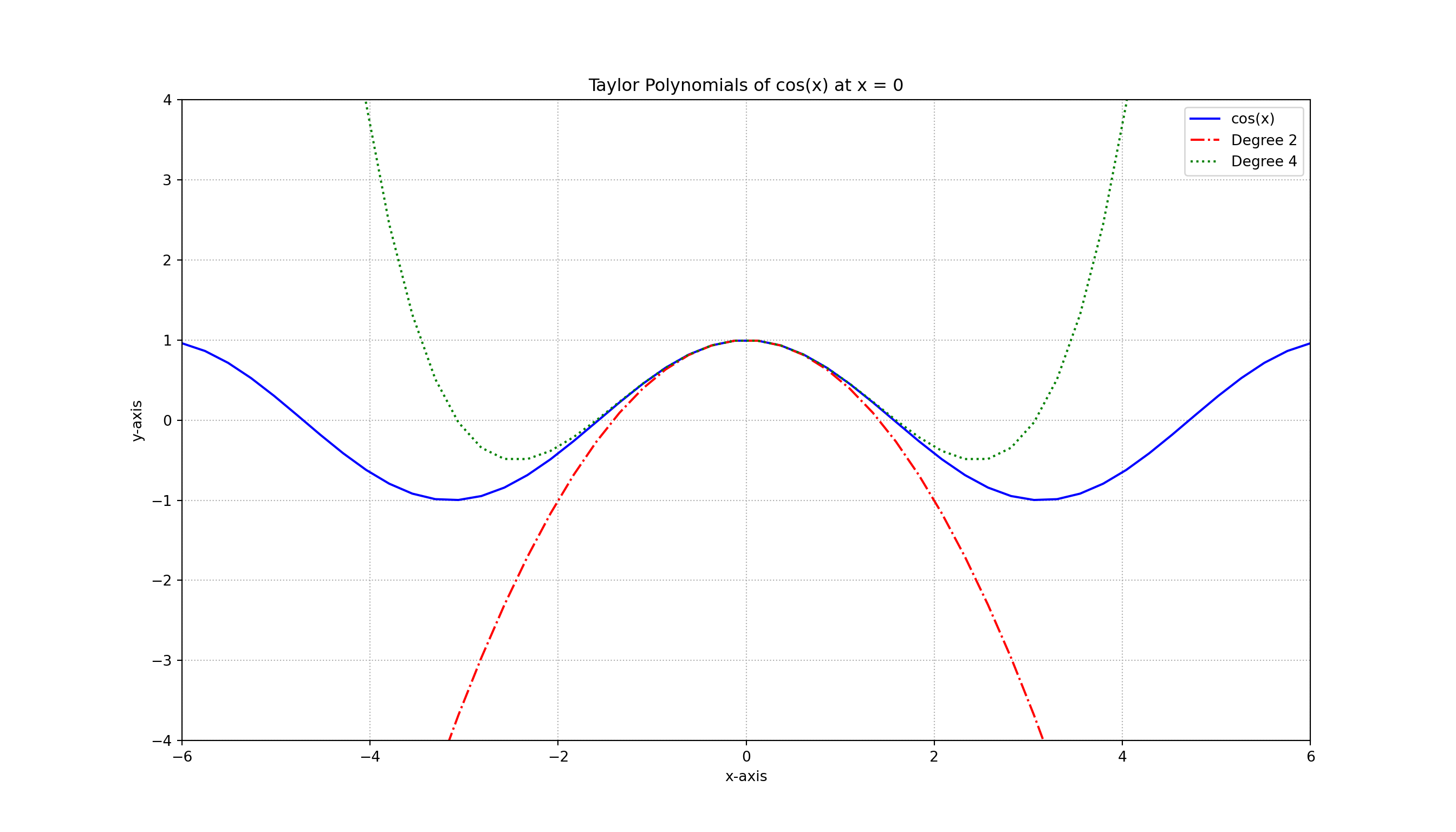
4.2 Functions with Latex labels
Python
# https://www.kaggle.com/sskiing/matplotlib-showcase-examples

import numpy as np
import matplotlib.pyplot as plt
from matplotlib.patches import Polygon

def func(x):
    return (x - 3) * (x - 5) * (x - 7) + 85

a, b = 2, 9  # integral limits
x = np.linspace(0, 10)
y = func(x)

fig, ax = plt.subplots(dpi=200)
plt.plot(x, y, 'r', linewidth=2)
plt.ylim(ymin=0)

# Make the shaded region
ix = np.linspace(a, b)
iy = func(ix)
verts = [(a, 0)] + list(zip(ix, iy)) + [(b, 0)]
poly = Polygon(verts, facecolor='0.9', edgecolor='0.5')
ax.add_patch(poly)

plt.text(0.5 * (a + b), 30, r"$\int_a^b f(x)\mathrm{d}x$",
         horizontalalignment='center', fontsize=20)

plt.figtext(0.9, 0.05, '$x$')
plt.figtext(0.1, 0.9, '$y$')

ax.spines['right'].set_visible(False)
ax.spines['top'].set_visible(False)
ax.xaxis.set_ticks_position('bottom')

ax.set_xticks((a, b))
ax.set_xticklabels(('$a$', '$b$'))
ax.set_yticks([])
plt.show()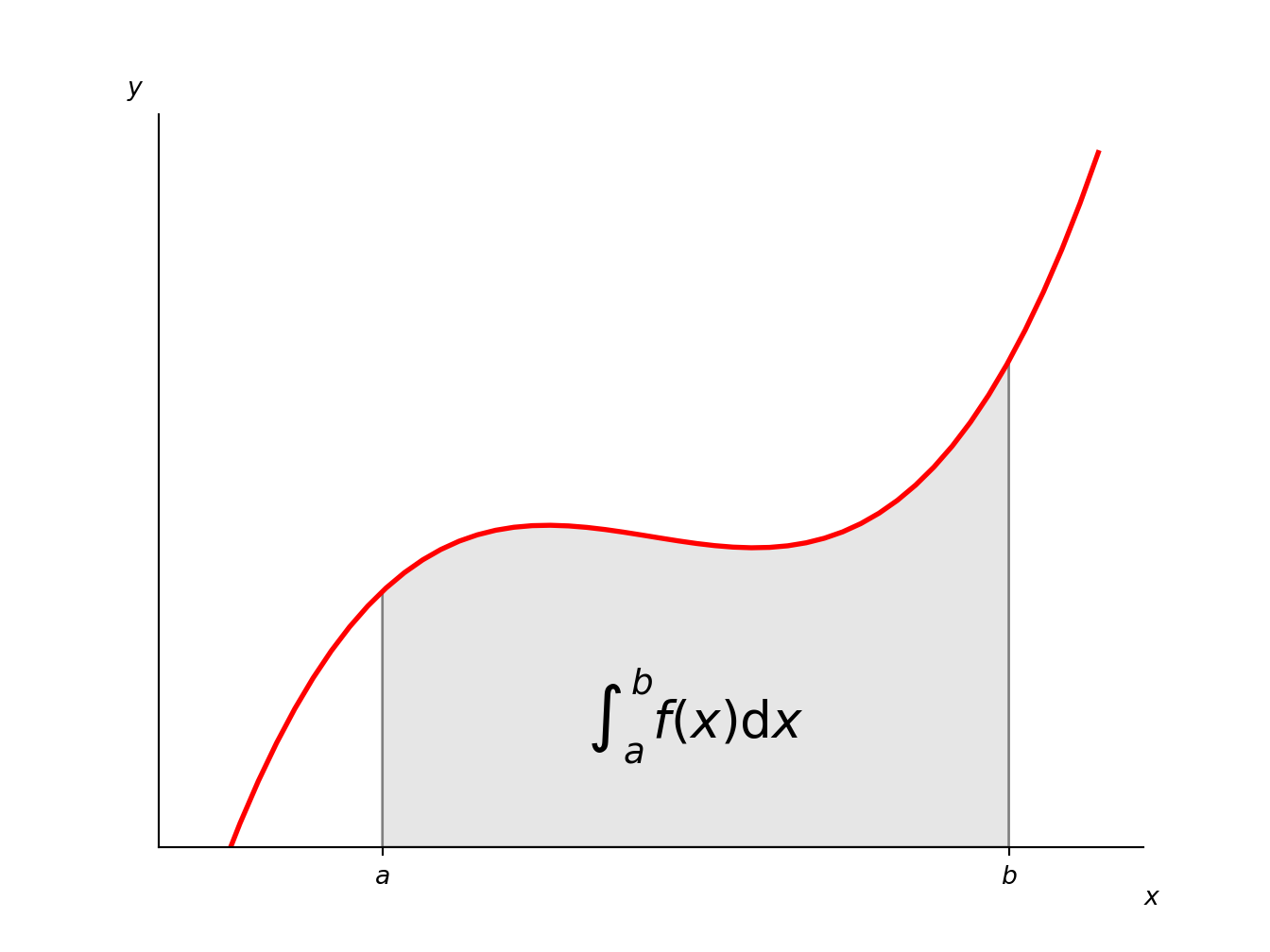
4.3 Multiple functions in the same plot
Python
import matplotlib.pyplot as plt
import numpy as np

t = np.arange(0.0, 2.0, 0.01)

s1 = np.sin(2 * np.pi * t)
s2 = np.exp(-t)
s3 = s1 * s2

fig, axs = plt.subplots(3, 1, sharex=True)
# Remove horizontal space between axes
fig.subplots_adjust(hspace=0)

# Plot each graph, and manually set the y tick values
axs[0].plot(t, s1)
axs[0].set_yticks(np.arange(-0.9, 1.0, 0.4))
axs[0].set_ylim(-1, 1)
axs[1].plot(t, s2)
axs[1].set_yticks(np.arange(0.1, 1.0, 0.2))
axs[1].set_ylim(0, 1)
axs[2].plot(t, s3)
axs[2].set_yticks(np.arange(-0.9, 1.0, 0.4))
axs[2].set_ylim(-1, 1)
plt.show()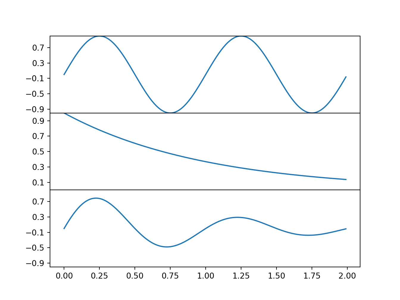
4.4 Overlapping functions
We use subplot to arrange the two functions. Observe that the y-axis is the same in both functions.
Python
# https://www.python-course.eu/matplotlib_multiple_figures.php
import numpy as np
import matplotlib.pyplot as plt
def f(t):
    return np.exp(-t) * np.cos(2*np.pi*t)
def g(t):
    return np.sin(t) * np.cos(1/(t+0.1))
t1 = np.arange(0.0, 5.0, 0.1)
t2 = np.arange(0.0, 5.0, 0.02)
plt.subplot(212)
plt.plot(t1, g(t1), 'ro', t2, f(t2), 'k')
plt.grid(color='b', alpha=0.5, linestyle='dashed', linewidth=0.5)
plt.show()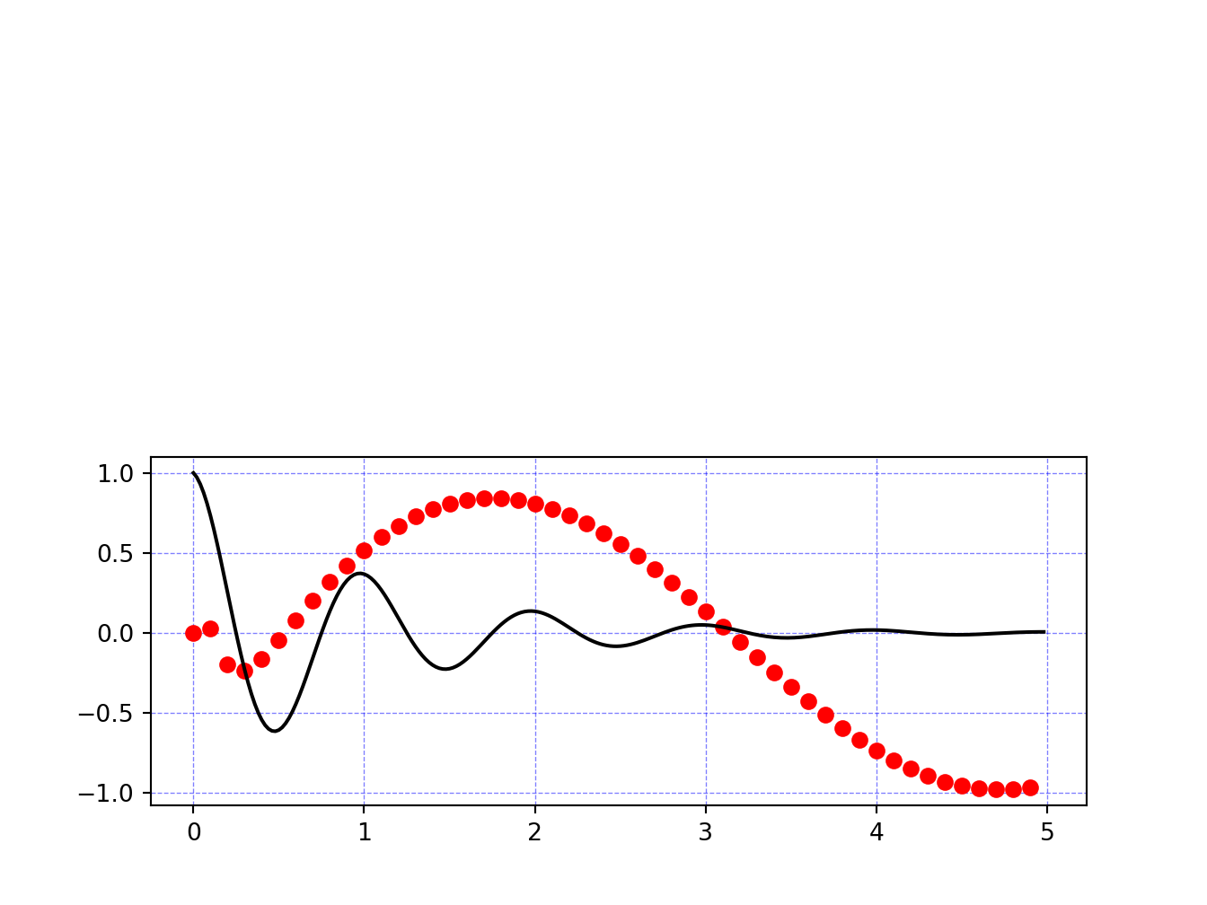
4.5 Surface functions
Python
# http://www.scipy-lectures.org/intro/matplotlib/auto_examples/plot_plot3d_ex.html
import numpy as np
import matplotlib.pyplot as plt
from mpl_toolkits.mplot3d import Axes3D

fig = plt.figure()
ax = Axes3D(fig)
X = np.arange(-4, 4, 0.25)
Y = np.arange(-4, 4, 0.25)
X, Y = np.meshgrid(X, Y)
R = np.sqrt(X ** 2 + Y ** 2)
Z = np.sin(R)

ax.plot_surface(X, Y, Z, rstride=1, cstride=1, cmap=plt.cm.hot)
ax.contourf(X, Y, Z, zdir='z', offset=-2, cmap=plt.cm.hot)
ax.set_zlim(-2, 2)
plt.show()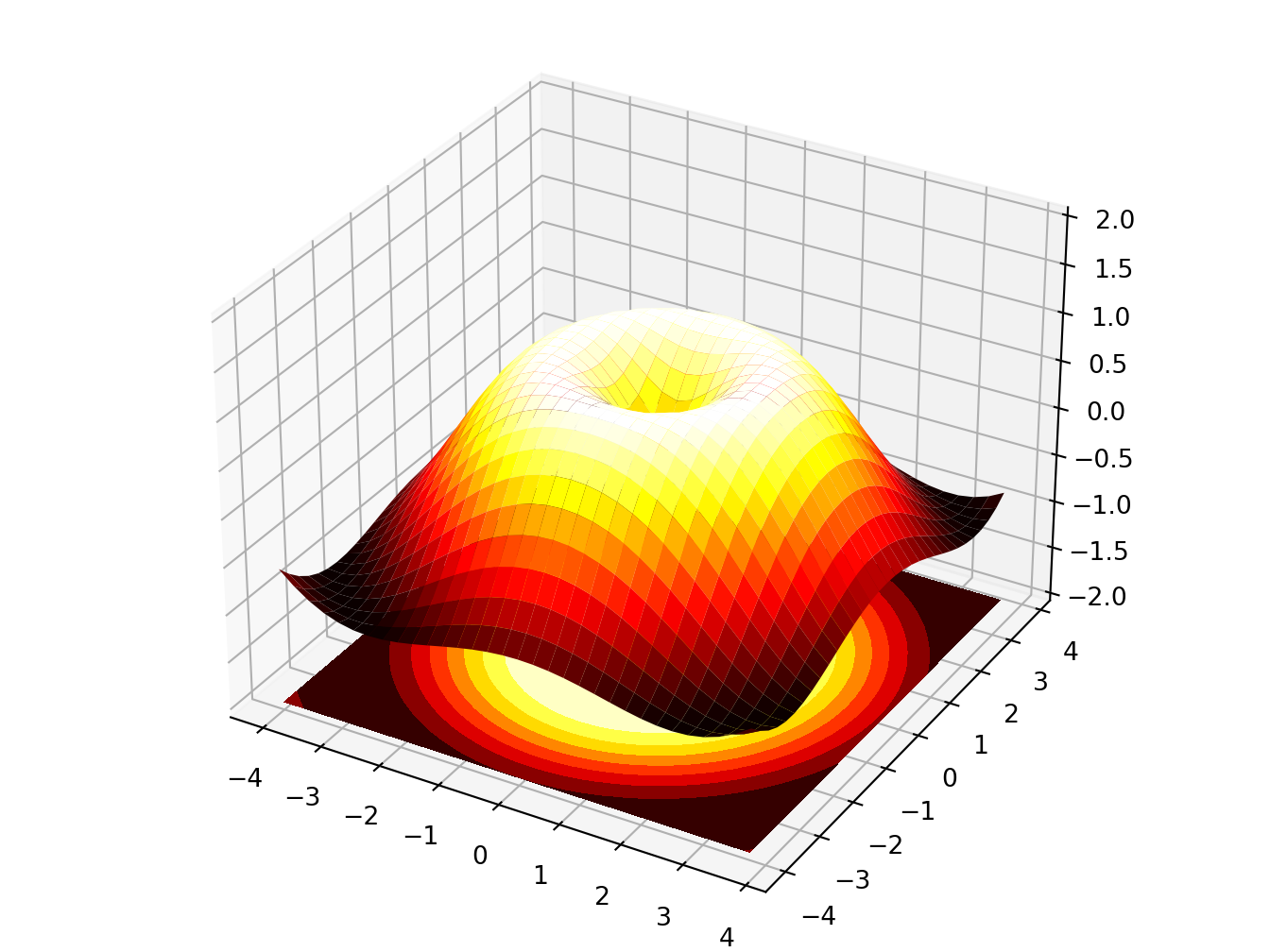
Python
# https://matplotlib.org/gallery/mplot3d/offset.html#sphx-glr-gallery-mplot3d-offset-py
# This import registers the 3D projection, but is otherwise unused.
from mpl_toolkits.mplot3d import Axes3D  # noqa: F401 unused import
import matplotlib.pyplot as plt
import numpy as np

fig = plt.figure()
ax = fig.gca(projection='3d')

X, Y = np.mgrid[0:6*np.pi:0.25, 0:4*np.pi:0.25]
Z = np.sqrt(np.abs(np.cos(X) + np.cos(Y)))

ax.plot_surface(X + 1e5, Y + 1e5, Z, cmap='autumn', cstride=2, rstride=2)

ax.set_xlabel("X label")
ax.set_ylabel("Y label")
ax.set_zlabel("Z label")
ax.set_zlim(0, 2)
plt.show()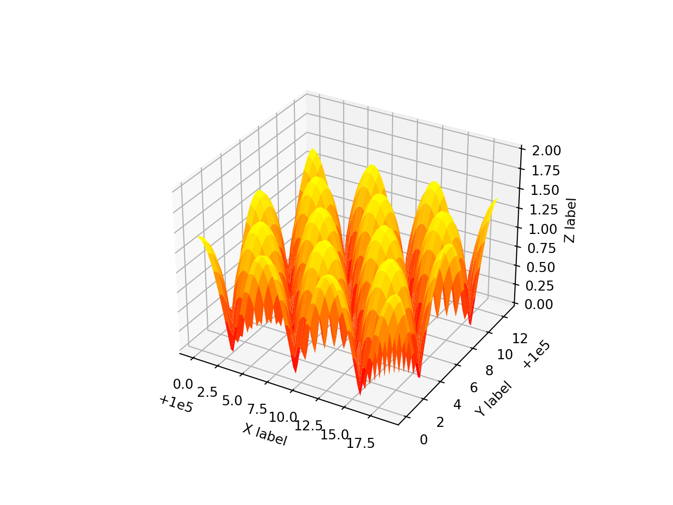
This is the typical example that you find in all Matlab books and tutorials.
Python
# https://github.com/matplotlib/matplotlib/blob/master/examples/mplot3d/surface3d_radial.py
from mpl_toolkits.mplot3d import Axes3D  # noqa: F401 unused import
import matplotlib.pyplot as plt
import numpy as np

fig = plt.figure()
ax = fig.add_subplot(111, projection='3d')

# Create the mesh in polar coordinates and compute corresponding Z.
r = np.linspace(0, 1.25, 50)
p = np.linspace(0, 2*np.pi, 50)
R, P = np.meshgrid(r, p)
Z = ((R**2 - 1)**2)
# Express the mesh in the cartesian system.
X, Y = R*np.cos(P), R*np.sin(P)
# Plot the surface.
ax.plot_surface(X, Y, Z, cmap=plt.cm.YlGnBu_r)
# Tweak the limits and add latex math labels.
ax.set_zlim(0, 1)
ax.set_xlabel(r'$\phi_\mathrm{real}$')
ax.set_ylabel(r'$\phi_\mathrm{im}$')
ax.set_zlabel(r'$V(\phi)$')

plt.show()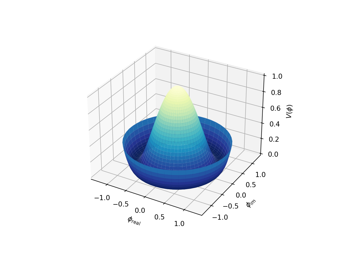
4.6 3D wireframe
Python
# https://github.com/matplotlib/matplotlib/blob/master/examples/mplot3d/wire3d.py
from mpl_toolkits.mplot3d import axes3d
import matplotlib.pyplot as plt

fig = plt.figure()
ax = fig.add_subplot(111, projection='3d')

# Grab some test data.
X, Y, Z = axes3d.get_test_data(0.05)

# Plot a basic wireframe.
ax.plot_wireframe(X, Y, Z, rstride=10, cstride=10)

plt.show()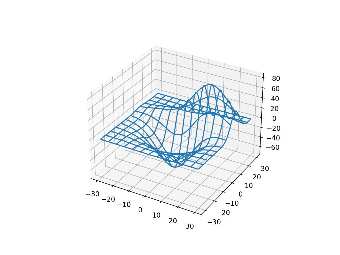
4.7 3D contour plot
Python
# https://matplotlib.org/2.0.2/examples/mplot3d/contour3d_demo.html
from mpl_toolkits.mplot3d import axes3d
import matplotlib.pyplot as plt
from matplotlib import cm

fig = plt.figure()
ax = fig.add_subplot(111, projection='3d')
X, Y, Z = axes3d.get_test_data(0.05)
cset = ax.contour(X, Y, Z, cmap=cm.coolwarm)
ax.clabel(cset, fontsize=9, inline=1)

plt.show()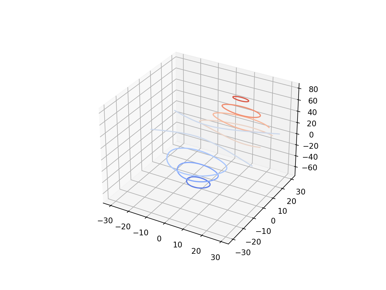
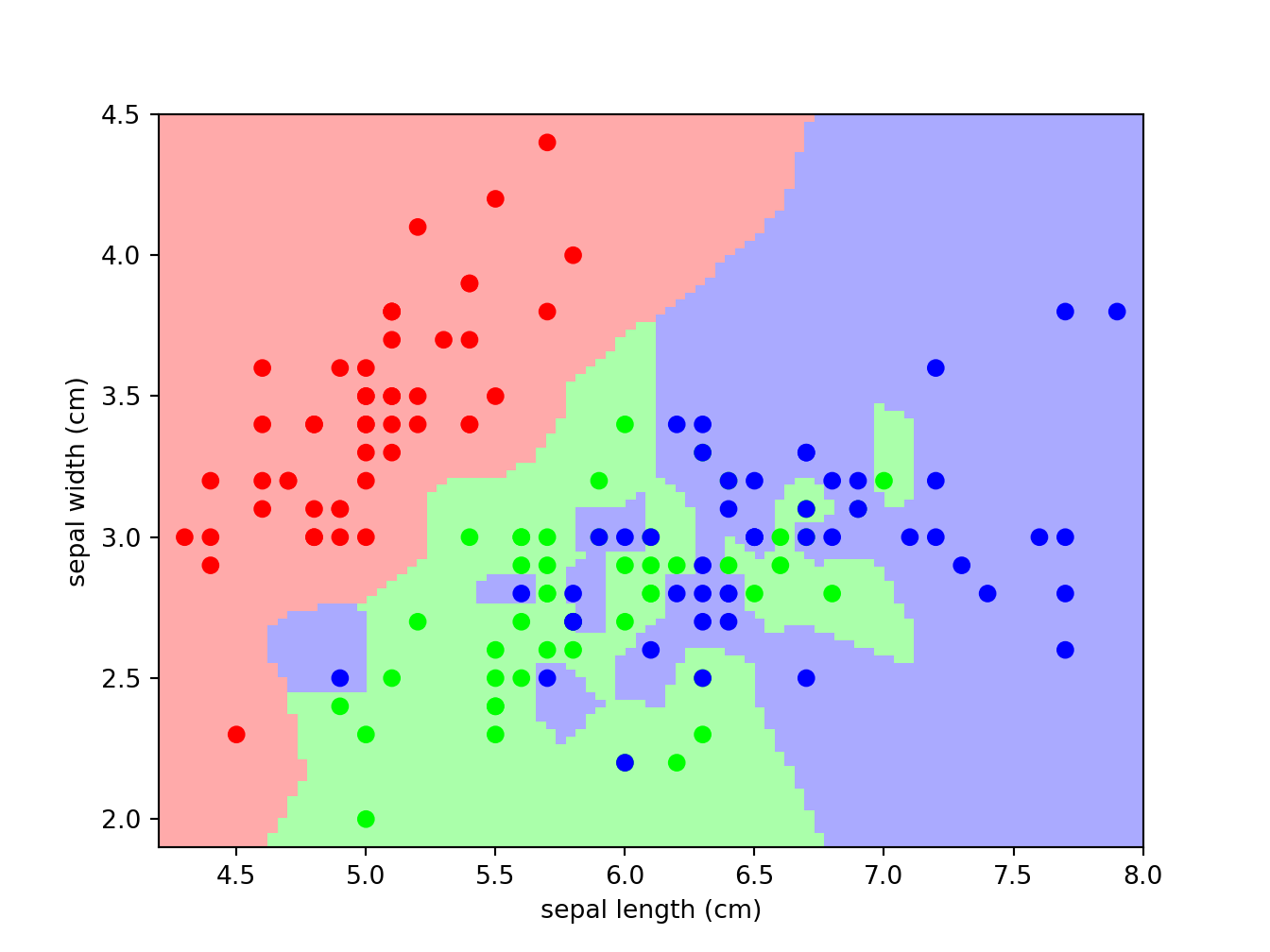
4.8 Machine Learning
This is just one sample of discovering patterns with machine learning.
Python
import numpy as np
from matplotlib import pyplot as plt
from sklearn import neighbors, datasets
from matplotlib.colors import ListedColormap

# Create color maps for 3-class classification problem, as with iris
cmap_light = ListedColormap(['#FFAAAA','#AAFFAA','#AAAAFF'])
cmap_bold = ListedColormap(['#FF0000','#00FF00','#0000FF'])

iris = datasets.load_iris()
X = iris.data[:, :2]  # we only take the first two features. We could
                      # avoid this ugly slicing by using a two-dim dataset
y = iris.target
knn = neighbors.KNeighborsClassifier(n_neighbors=1)
knn.fit(X, y)
x_min, x_max = X[:, 0].min() - .1, X[:, 0].max() + .1
y_min, y_max = X[:, 1].min() - .1, X[:, 1].max() + .1
xx, yy = np.meshgrid(np.linspace(x_min, x_max, 100), np.linspace(y_min, y_max, 100))

Z = knn.predict(np.c_[xx.ravel(), yy.ravel()])

Z = Z.reshape(xx.shape)
plt.figure()
plt.pcolormesh(xx, yy, Z, cmap=cmap_light)

# Plot also the training points
plt.scatter(X[:, 0], X[:, 1], c=y, cmap=cmap_bold)
plt.xlabel('sepal length (cm)')
plt.ylabel('sepal width (cm)')
plt.axis('tight')
plt.show()