Papp correlation

(Hall and Yarborough 1973) This is an explicit correlation by I. Papp (Papp 1979) mentioned in the comparative analysis paper by Gabor Takacs (Takacs 1989). The original paper is not available in English but Prof. Takacs describe the equation in his paper of 1989.

Get `z` at selected `Ppr` and `Tpr`

Use the the correlation to calculate z and from Standing-Katz chart obtain z a digitized point at the given Tpr and Ppr.

# get a z value
library(zFactor)
ppr <- 1.5
tpr <- 2.0

z.calc <- z.Papp(pres.pr = ppr, temp.pr = tpr)

# get a z value from the SK chart at the same Ppr and Tpr
z.chart <- getStandingKatzMatrix(tpr_vector = tpr, 
                      pprRange = "lp")[1, as.character(ppr)]

# calculate the APE
ape <- abs((z.calc - z.chart) / z.chart) * 100

df <- as.data.frame(list(Ppr = ppr,  z.calc =z.calc, z.chart = z.chart, ape=ape))
rownames(df) <- tpr
df
# HY = 0.9580002; # DAK = 0.9551087

  Ppr   z.calc z.chart       ape
2 1.5 0.962332   0.956 0.6623461

Get `z` at selected `Ppr` and `Tpr=1.1`

From the Standing-Katz chart we read z at a digitized point:

library(zFactor)
ppr <- 1.5
tpr <- 1.1

z.calc <- z.Papp(pres.pr = ppr, temp.pr = tpr)

# From the Standing-Katz chart we obtain a digitized point:
z.chart <- getStandingKatzMatrix(tpr_vector = tpr, 
                      pprRange = "lp")[1, as.character(ppr)]

# calculate the APE (Average Percentage Error)
ape <- abs((z.calc - z.chart) / z.chart) * 100

df <- as.data.frame(list(Ppr = ppr,  z.calc =z.calc, z.chart = z.chart, ape=ape))
rownames(df) <- tpr
df
# HY = 0.4732393  APE = 11.08903

    Ppr    z.calc z.chart      ape
1.1 1.5 0.5361425   0.426 25.85506

Get values of `z` for combinations of `Ppr` and `Tpr`

In this example we provide vectors instead of a single point. With the same ppr and tpr vectors that we use for the correlation, we do the same for the Standing-Katz chart. We want to compare both and find the absolute percentage error or APE.

# test with vector extracted from paper
ppr <- c(0.5, 1.5, 2.5, 3.5, 4.5, 5.5, 6.5) 
tpr <- c(1.05, 1.1, 1.7, 2) 

# calculate using the correlation
z.calc <- z.Papp(ppr, tpr)

# With the same ppr and tpr vector, we do the same for the Standing-Katz chart
z.chart <- getStandingKatzMatrix(ppr_vector = ppr, tpr_vector = tpr)
ape <- abs((z.calc - z.chart) / z.chart) * 100

# calculate the APE
cat("z.correlation \n"); print(z.calc)
cat("\n z.chart \n"); print(z.chart)
cat("\n APE \n"); print(ape)

z.correlation 
           0.5       1.5       2.5       3.5       4.5       5.5       6.5
1.05 0.8243607 0.4692711 0.3958632 0.4788553 0.5906236 0.7046099 0.8186716
1.1  0.8517120 0.5361425 0.4430332 0.5056550 0.6077642 0.7145435 0.8215955
1.7  0.9736623 0.9138939 0.8665932 0.8471834 0.8578133 0.8919610 0.9406180
2    0.9877275 0.9623320 0.9432543 0.9366532 0.9450048 0.9675653 1.0015334

 z.chart 
       0.5   1.5   2.5   3.5   4.5   5.5   6.5
1.05 0.829 0.253 0.343 0.471 0.598 0.727 0.846
1.10 0.854 0.426 0.393 0.500 0.615 0.729 0.841
1.70 0.968 0.914 0.876 0.857 0.864 0.897 0.942
2.00 0.982 0.956 0.941 0.937 0.945 0.969 1.003

 APE 
           0.5         1.5        2.5        3.5         4.5       5.5
1.05 0.5596238 85.48266650 15.4120172 1.66779568 1.233507926 3.0797870
1.1  0.2679163 25.85505860 12.7311015 1.13099950 1.176554761 1.9830566
1.7  0.5849433  0.01160694  1.0738373 1.14546413 0.716057626 0.5617635
2    0.5832436  0.66234608  0.2395608 0.03701248 0.000507908 0.1480622
           6.5
1.05 3.2303092
1.1  2.3073158
1.7  0.1467143
2    0.1462221

Analyze the error at the `isotherms`

Applying the function summary over the transpose of the matrix:

sum_t_ape <- summary(t(ape))
sum_t_ape

      1.05              1.1               1.7                2            
 Min.   : 0.5596   Min.   : 0.2679   Min.   :0.01161   Min.   :0.0005079  
 1st Qu.: 1.4506   1st Qu.: 1.1538   1st Qu.:0.35424   1st Qu.:0.0916173  
 Median : 3.0798   Median : 1.9831   Median :0.58494   Median :0.1480622  
 Mean   :15.8094   Mean   : 6.4931   Mean   :0.60577   Mean   :0.2595650  
 3rd Qu.: 9.3212   3rd Qu.: 7.5192   3rd Qu.:0.89495   3rd Qu.:0.4114022  
 Max.   :85.4827   Max.   :25.8551   Max.   :1.14546   Max.   :0.6623461

Analyze the error for greater values of `Tpr`

library(zFactor)
# enter vectors for Tpr and Ppr
tpr2 <- c(1.2, 1.3, 1.5, 2.0, 3.0) 
ppr2 <- c(0.5, 1.5, 2.5, 3.5, 4.5, 5.5) 

# get z values from the SK chart
z.chart <- getStandingKatzMatrix(ppr_vector = ppr2, tpr_vector = tpr2, pprRange = "lp")

# We do the same with the HY correlation:
# calculate z values at lower values of Tpr
z.calc <- z.Papp(pres.pr = ppr2, temp.pr = tpr2) 
ape <- abs((z.calc - z.chart) / z.chart) * 100

# calculate the APE
cat("z.correlation \n"); print(z.calc)
cat("\n z.chart \n"); print(z.chart)
cat("\n APE \n"); print(ape)

z.correlation 
          0.5       1.5       2.5       3.5       4.5       5.5
1.2 0.8926577 0.6489440 0.5388870 0.5640639 0.6449346 0.7382795
1.3 0.9208943 0.7357072 0.6290383 0.6271826 0.6858996 0.7656800
1.5 0.9552137 0.8499334 0.7728520 0.7501411 0.7749505 0.8279008
2   0.9877275 0.9623320 0.9432543 0.9366532 0.9450048 0.9675653
3   0.9995561 1.0001483 1.0032952 1.0095589 1.0193297 1.0328185

 z.chart 
       0.5   1.5   2.5   3.5   4.5   5.5
1.20 0.893 0.657 0.519 0.565 0.650 0.741
1.30 0.916 0.756 0.638 0.633 0.684 0.759
1.50 0.948 0.859 0.794 0.770 0.790 0.836
2.00 0.982 0.956 0.941 0.937 0.945 0.969
3.00 1.002 1.009 1.018 1.029 1.041 1.056

 APE 
           0.5       1.5       2.5        3.5         4.5       5.5
1.2 0.03832749 1.2261856 3.8317839 0.16567267 0.779298982 0.3671385
1.3 0.53431458 2.6842320 1.4046605 0.91901585 0.277717125 0.8801037
1.5 0.76093659 1.0554821 2.6634712 2.57908019 1.905004145 0.9688092
2   0.58324362 0.6623461 0.2395608 0.03701248 0.000507908 0.1480622
3   0.24389752 0.8772760 1.4444808 1.88931540 2.081676730 2.1952223

Analyze the error at the `isotherms`

Applying the function summary over the transpose of the matrix to observe the error of the correlation at each isotherm.

sum_t_ape <- summary(t(ape))
sum_t_ape
 # Hall-Yarborough
 #      1.2               1.3              1.5               2         
 # Min.   :0.05224   Min.   :0.1105   Min.   :0.1021   Min.   :0.0809  
 # 1st Qu.:0.09039   1st Qu.:0.2080   1st Qu.:0.1623   1st Qu.:0.1814  
 # Median :0.28057   Median :0.3181   Median :0.1892   Median :0.1975  
 # Mean   :0.30122   Mean   :0.3899   Mean   :0.2597   Mean   :0.2284  
 # 3rd Qu.:0.51710   3rd Qu.:0.5355   3rd Qu.:0.3533   3rd Qu.:0.2627  
 # Max.   :0.57098   Max.   :0.8131   Max.   :0.5162   Max.   :0.4338  
 #       3          
 # Min.   :0.09128  
 # 1st Qu.:0.17466  
 # Median :0.35252  
 # Mean   :0.34820  
 # 3rd Qu.:0.52184  
 # Max.   :0.59923

      1.2               1.3              1.5               2            
 Min.   :0.03833   Min.   :0.2777   Min.   :0.7609   Min.   :0.0005079  
 1st Qu.:0.21604   1st Qu.:0.6208   1st Qu.:0.9905   1st Qu.:0.0647749  
 Median :0.57322   Median :0.8996   Median :1.4802   Median :0.1938115  
 Mean   :1.06807   Mean   :1.1167   Mean   :1.6555   Mean   :0.2784555  
 3rd Qu.:1.11446   3rd Qu.:1.2832   3rd Qu.:2.4106   3rd Qu.:0.4973229  
 Max.   :3.83178   Max.   :2.6842   Max.   :2.6635   Max.   :0.6623461  
       3         
 Min.   :0.2439  
 1st Qu.:1.0191  
 Median :1.6669  
 Mean   :1.4553  
 3rd Qu.:2.0336  
 Max.   :2.1952

Prepare to plot SK vs PP correlation

library(zFactor)
library(tibble)
library(ggplot2)

tpr2 <- c(1.05, 1.1, 1.2, 1.3) 
ppr2 <- c(0.5, 1.0, 1.5, 2, 2.5, 3.0, 3.5, 4.0, 4.5, 5.0, 5.5, 6.0, 6.5) 

sk_dak_2 <- createTidyFromMatrix(ppr2, tpr2, correlation = "PP")
as_tibble(sk_dak_2)

p <- ggplot(sk_dak_2, aes(x=Ppr, y=z.calc, group=Tpr, color=Tpr)) +
    geom_line() +
    geom_point() +
    geom_errorbar(aes(ymin=z.calc-dif, ymax=z.calc+dif), width=.4,
                  position=position_dodge(0.05))
print(p)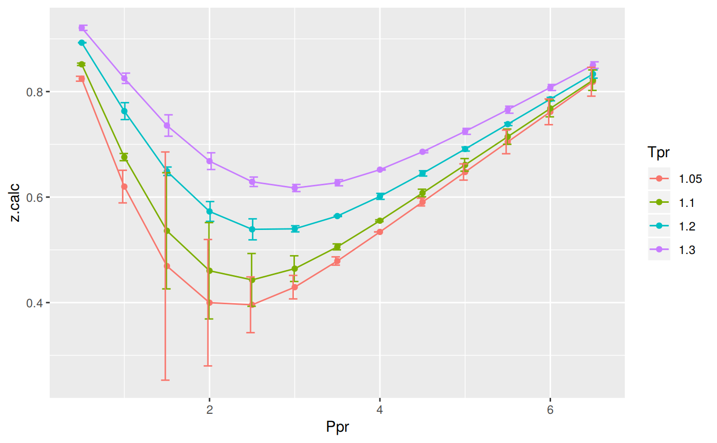

# A tibble: 52 x 5
   Tpr     Ppr z.chart z.calc       dif
   <chr> <dbl>   <dbl>  <dbl>     <dbl>
 1 1.05    0.5   0.829  0.824  0.00464 
 2 1.1     0.5   0.854  0.852  0.00229 
 3 1.2     0.5   0.893  0.893  0.000342
 4 1.3     0.5   0.916  0.921 -0.00489 
 5 1.05    1     0.589  0.620 -0.0309  
 6 1.1     1     0.669  0.676 -0.00680 
 7 1.2     1     0.779  0.763  0.0160  
 8 1.3     1     0.835  0.825  0.00981 
 9 1.05    1.5   0.253  0.469 -0.216   
10 1.1     1.5   0.426  0.536 -0.110   
# … with 42 more rows

Analysis at the lowest `Tpr`

This is the isotherm where we see the greatest error.

library(zFactor)

sk_dak_3 <- sk_dak_2[sk_dak_2$Tpr==1.05,]
sk_dak_3

p <- ggplot(sk_dak_3, aes(x=Ppr, y=z.calc, group=Tpr, color=Tpr)) +
    geom_line() +
    geom_point() +
    geom_errorbar(aes(ymin=z.calc-dif, ymax=z.calc+dif), width=.2,
                  position=position_dodge(0.05))
print(p)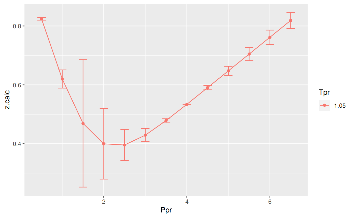

    Tpr Ppr z.chart    z.calc           dif
1  1.05 0.5   0.829 0.8243607  4.639281e-03
5  1.05 1.0   0.589 0.6199052 -3.090525e-02
9  1.05 1.5   0.253 0.4692711 -2.162711e-01
13 1.05 2.0   0.280 0.3998218 -1.198218e-01
17 1.05 2.5   0.343 0.3958632 -5.286322e-02
21 1.05 3.0   0.407 0.4292515 -2.225150e-02
25 1.05 3.5   0.471 0.4788553 -7.855318e-03
29 1.05 4.0   0.534 0.5339879  1.210687e-05
33 1.05 4.5   0.598 0.5906236  7.376377e-03
37 1.05 5.0   0.663 0.6475878  1.541217e-02
41 1.05 5.5   0.727 0.7046099  2.239005e-02
45 1.05 6.0   0.786 0.7616403  2.435970e-02
49 1.05 6.5   0.846 0.8186716  2.732842e-02

Analyzing performance of the `PP` correlation for all the `Tpr` curves

In this last example, we compare the values of z at all the isotherms.

We use the function getCurvesDigitized to obtain all the isotherms or Tpr curves in the Standing-Katz chart that have been digitized.

The next function createTidyFromMatrix calculates z using the correlation and prepares a tidy dataset ready to plot.

library(ggplot2)
library(tibble)

# get all `lp` Tpr curves
tpr_all <- getStandingKatzTpr(pprRange = "lp")
ppr <- c(0.5, 1.5, 2.5, 3.5, 4.5, 5.5, 6.5) 
sk_corr_all <- createTidyFromMatrix(ppr, tpr_all, correlation = "PP")
as_tibble(sk_corr_all)

p <- ggplot(sk_corr_all, aes(x=Ppr, y=z.calc, group=Tpr, color=Tpr)) +
    geom_line() +
    geom_point() +
    geom_errorbar(aes(ymin=z.calc-dif, ymax=z.calc+dif), width=.4,
                  position=position_dodge(0.05))
print(p)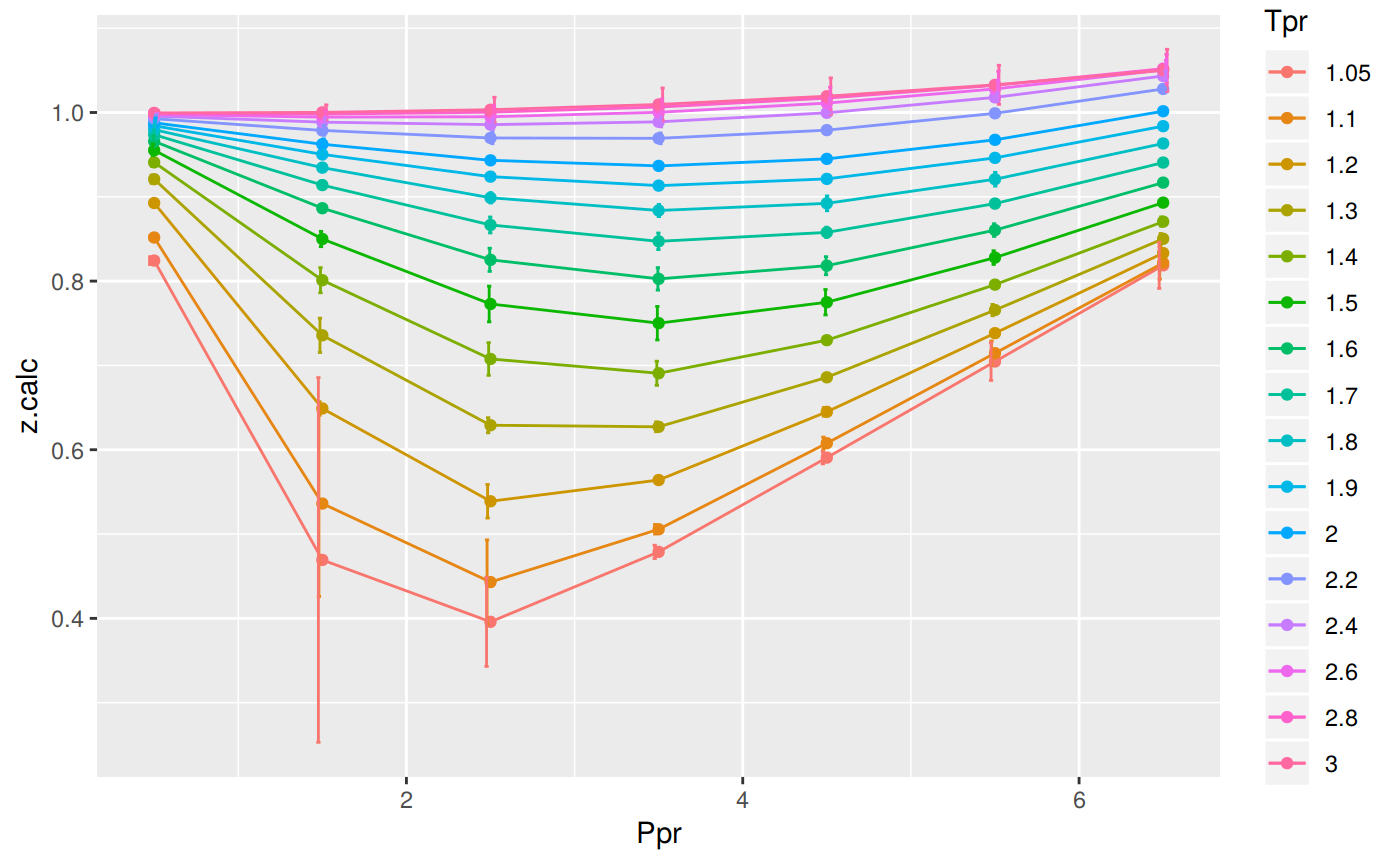

# A tibble: 112 x 5
   Tpr     Ppr z.chart z.calc       dif
   <chr> <dbl>   <dbl>  <dbl>     <dbl>
 1 1.05    0.5   0.829  0.824  0.00464 
 2 1.1     0.5   0.854  0.852  0.00229 
 3 1.2     0.5   0.893  0.893  0.000342
 4 1.3     0.5   0.916  0.921 -0.00489 
 5 1.4     0.5   0.936  0.941 -0.00483 
 6 1.5     0.5   0.948  0.955 -0.00721 
 7 1.6     0.5   0.959  0.966 -0.00678 
 8 1.7     0.5   0.968  0.974 -0.00566 
 9 1.8     0.5   0.974  0.980 -0.00563 
10 1.9     0.5   0.978  0.984 -0.00620 
# … with 102 more rows

Range of applicability of the correlation

# MSE: Mean Squared Error
# RMSE: Root Mean Squared Error
# RSS: residual sum of square
# ARE:  Average Relative Error, %
# AARE: Average Absolute Relative Error, %
library(dplyr)
grouped <- group_by(sk_corr_all, Tpr, Ppr)

smry_tpr_ppr <- summarise(grouped, 
          RMSE= sqrt(mean((z.chart-z.calc)^2)), 
          MPE = sum((z.calc - z.chart) / z.chart) * 100 / n(),
          MAPE = sum(abs((z.calc - z.chart) / z.chart)) * 100 / n(), 
          MSE = sum((z.calc - z.chart)^2) / n(), 
          RSS = sum((z.calc - z.chart)^2),
          MAE = sum(abs(z.calc - z.chart)) / n(),
          RMLSE = sqrt(1/n()*sum((log(z.calc +1)-log(z.chart +1))^2))
          )

ggplot(smry_tpr_ppr, aes(Ppr, Tpr)) + 
    geom_tile(data=smry_tpr_ppr, aes(fill=MAPE), color="white") +
    scale_fill_gradient2(low="blue", high="red", mid="yellow", na.value = "pink",
                         midpoint=12.5, limit=c(0, 25), name="MAPE") + 
    theme(axis.text.x = element_text(angle=45, vjust=1, size=11, hjust=1)) + 
    coord_equal() +
    ggtitle("Papp", subtitle = "PP")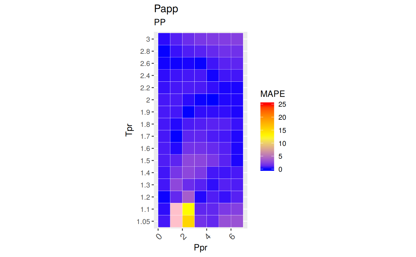

Plotting the `Tpr` and `Ppr` values that show more error

The MAPE (mean average percentage error) gradient bar indicates that the more red the square is, the more error there is.

library(dplyr)

sk_corr_all %>%
    filter(Tpr %in% c("1.05", "1.1", "1.2", "2.6", "2.8", "3")) %>%
    ggplot(aes(x = z.chart, y=z.calc, group = Tpr, color = Tpr)) +
    geom_point(size = 3) +
    geom_line(aes(x = z.chart, y = z.chart), color = "black") +
    facet_grid(. ~ Tpr, scales = "free") +
    geom_errorbar(aes(ymin=z.calc-abs(dif), ymax=z.calc+abs(dif)), 
                  position=position_dodge(0.5))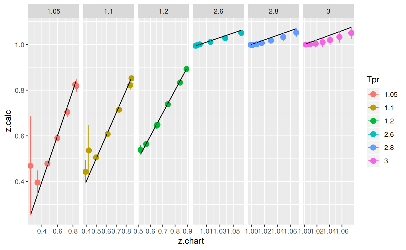

With the exception of the isotherms at 1.05 and 1.1, the Papp correlation looks acceptable good.

Looking numerically at the errors

Finally, the dataframe with the calculated errors between the z from the correlation and the z read from the chart:

as_tibble(smry_tpr_ppr)

# A tibble: 112 x 9
   Tpr     Ppr    RMSE    MPE   MAPE        MSE        RSS     MAE   RMLSE
   <chr> <dbl>   <dbl>  <dbl>  <dbl>      <dbl>      <dbl>   <dbl>   <dbl>
 1 1.05    0.5 0.00464 -0.560  0.560 0.0000215  0.0000215  0.00464 0.00254
 2 1.05    1.5 0.216   85.5   85.5   0.0468     0.0468     0.216   0.159  
 3 1.05    2.5 0.0529  15.4   15.4   0.00279    0.00279    0.0529  0.0386 
 4 1.05    3.5 0.00786  1.67   1.67  0.0000617  0.0000617  0.00786 0.00533
 5 1.05    4.5 0.00738 -1.23   1.23  0.0000544  0.0000544  0.00738 0.00463
 6 1.05    5.5 0.0224  -3.08   3.08  0.000501   0.000501   0.0224  0.0130 
 7 1.05    6.5 0.0273  -3.23   3.23  0.000747   0.000747   0.0273  0.0149 
 8 1.1     0.5 0.00229 -0.268  0.268 0.00000523 0.00000523 0.00229 0.00123
 9 1.1     1.5 0.110   25.9   25.9   0.0121     0.0121     0.110   0.0744 
10 1.1     2.5 0.0500  12.7   12.7   0.00250    0.00250    0.0500  0.0353 
# … with 102 more rows

References

Hall, Kenneth R, and Lyman Yarborough. 1973. “A New Equation of State for Z-Factor Calculations.” Oil and Gas Journal 71 (7): 82–92.

Papp, I. 1979. “Uj Modszer Foldgazok Elteresi Tenyezojenek Szamitasara.” Koolaj Es Foldgaz, November, 345–47.

Takacs, Gabor. 1989. “Comparing Methods for Calculating Z Factor.” Oil and Gas Journal, May. Oil; Gas Journal. https://www.researchgate.net/publication/236510717_Comparing_methods_for_calculating_Z-factor.

Papp correlation

2019-08-01