Dranchuk-Purvis-Robinson correlation

2019-08-01

Why DPR is different

The Dranchuk-Purvis-Robinson correlation is different than the other correlations in the sense that the authors were looking at redrawing three of the isotherms of the original work by Standing-Katz: the curves at Tpr=1.05, Tpr=1.1 and Tpr=1.15. The authors were expecting that later the corrections to be adopted with experimental data matching those two new curves. We haven’t found a paper confirming that yet. (See Dranchuk et al. 1973).

Other than that, the DPR correlation behaves pretty well but not much better than the DAK correlation.

Get z at selected Ppr and Tpr

Use the corelation to calculate z. From the Standing-Katz chart we obtain z at a digitized point at the given Tpr and Ppr.

# get a z value
library(zFactor)

ppr <- 1.5
tpr <- 2.0

z.calc <- z.DranchukPurvisRobinson(pres.pr = ppr, temp.pr = tpr)

# get a z value from the SK chart at the same Ppr and Tpr
z.chart <- getStandingKatzMatrix(tpr_vector = tpr, 
                      pprRange = "lp")[1, as.character(ppr)]

# calculate the APE
ape <- abs((z.calc - z.chart) / z.chart) * 100

df <- as.data.frame(list(Ppr = ppr,  z.calc =z.calc, z.chart = z.chart, ape=ape))
rownames(df) <- tpr
df
# HY = 0.9580002; # DAK = 0.9551087

  Ppr    z.calc z.chart       ape
2 1.5 0.9546382   0.956 0.1424501

Get z at selected Ppr and Tpr=1.1

From the Standing-Katz chart we obtain z at a digitized point:

library(zFactor)

ppr <- 1.5
tpr <- 1.1
z.calc <- z.DranchukPurvisRobinson(pres.pr = ppr, temp.pr = tpr)

# From the Standing-Katz chart we obtain a digitized point:
z.chart <- getStandingKatzMatrix(tpr_vector = tpr, 
                      pprRange = "lp")[1, as.character(ppr)]

# calculate the APE
ape <- abs((z.calc - z.chart) / z.chart) * 100

df <- as.data.frame(list(Ppr = ppr,  z.calc =z.calc, z.chart = z.chart, ape=ape))
rownames(df) <- tpr
df

    Ppr    z.calc z.chart      ape
1.1 1.5 0.4429389   0.426 3.976272

At lower Tpr we can see that there is some difference between the values of z from the DPR calculation and the value read from the Standing-Katz chart.

Get values of z for combinations of Ppr and Tpr

In this example we provide vectors instead of a single point. With the same ppr and tpr vectors that we use for the correlation, we do the same for the Standing-Katz chart. We want to compare both and find the absolute percentage error.

# test HY with 1st-derivative using the values from paper 
ppr <- c(0.5, 1.5, 2.5, 3.5, 4.5, 5.5, 6.5) 
tpr <- c(1.05, 1.1, 1.7, 2) 

# calculate using the correlation
z.calc <- z.DranchukPurvisRobinson(ppr, tpr)

# With the same ppr and tpr vector, we do the same for the Standing-Katz chart
z.chart <- getStandingKatzMatrix(ppr_vector = ppr, tpr_vector = tpr)
ape <- abs((z.calc - z.chart) / z.chart) * 100

# calculate the APE
cat("z.correlation \n"); print(z.calc)
cat("\n z.chart \n"); print(z.chart)
cat("\n APE \n"); print(ape)

z.correlation 
           0.5       1.5       2.5       3.5       4.5       5.5       6.5
1.05 0.8299757 0.2849670 0.3874732 0.5071451 0.6251306 0.7407256 0.8540945
1.1  0.8566368 0.4429389 0.4120547 0.5173680 0.6278497 0.7376397 0.8458855
1.7  0.9677844 0.9121791 0.8752677 0.8630002 0.8743271 0.9033216 0.9440582
2    0.9822021 0.9546382 0.9399310 0.9391490 0.9512966 0.9740256 1.0047347

 z.chart 
       0.5   1.5   2.5   3.5   4.5   5.5   6.5
1.05 0.829 0.253 0.343 0.471 0.598 0.727 0.846
1.10 0.854 0.426 0.393 0.500 0.615 0.729 0.841
1.70 0.968 0.914 0.876 0.857 0.864 0.897 0.942
2.00 0.982 0.956 0.941 0.937 0.945 0.969 1.003

 APE 
            0.5        1.5         2.5       3.5       4.5       5.5
1.05 0.11769033 12.6351920 12.96594664 7.6741203 4.5368917 1.8879838
1.1  0.30875526  3.9762721  4.84851814 3.4735929 2.0893900 1.1851375
1.7  0.02227128  0.1992260  0.08360117 0.7001396 1.1952693 0.7047482
2    0.02057809  0.1424501  0.11359921 0.2293483 0.6663029 0.5186423
           6.5
1.05 0.9567950
1.1  0.5809181
1.7  0.2184874
2    0.1729508

You can see errors of 12.64% and 12.97% in the isotherm Tpr=1.05. Other errors, greater than one, can also be found at the isotherm Tpr=1.1: 4.85%. Then, the rest of the Tpr curves are fine.

Analyze the error at the isotherms

Applying the function summary over the transpose of the matrix:

sum_t_ape <- summary(t(ape))
sum_t_ape

      1.05              1.1              1.7                2          
 Min.   : 0.1177   Min.   :0.3088   Min.   :0.02227   Min.   :0.02058  
 1st Qu.: 1.4224   1st Qu.:0.8830   1st Qu.:0.14141   1st Qu.:0.12802  
 Median : 4.5369   Median :2.0894   Median :0.21849   Median :0.17295  
 Mean   : 5.8249   Mean   :2.3518   Mean   :0.44625   Mean   :0.26627  
 3rd Qu.:10.1547   3rd Qu.:3.7249   3rd Qu.:0.70244   3rd Qu.:0.37400  
 Max.   :12.9659   Max.   :4.8485   Max.   :1.19527   Max.   :0.66630  

We see that the errors at Tpr=1.05 in z are considerable with a Min. : 0.1177 % and Max. :12.9659 %, and a Min. :0.3088 % and Max. :4.8485 % for Tpr=1.10. We will explore later a comparative tile chart where we confirm these early calculations.

Analyze the error for greater values of Tpr

library(zFactor)
# enter vectors for Tpr and Ppr
tpr2 <- c(1.2, 1.3, 1.5, 2.0, 3.0) 
ppr2 <- c(0.5, 1.5, 2.5, 3.5, 4.5, 5.5) 
# get z values from the SK chart
z.chart <- getStandingKatzMatrix(ppr_vector = ppr2, tpr_vector = tpr2, pprRange = "lp")

# We do the same with the DPR correlation:
# calculate z values at lower values of Tpr
z.calc <- z.DranchukPurvisRobinson(pres.pr = ppr2, temp.pr = tpr2) 
ape <- abs((z.calc - z.chart) / z.chart) * 100

# calculate the APE
cat("z.correlation \n"); print(z.calc)
cat("\n z.chart \n"); print(z.chart)
cat("\n APE \n"); print(ape)

z.correlation 
          0.5       1.5       2.5       3.5       4.5       5.5
1.2 0.8944622 0.6506542 0.5167723 0.5620069 0.6486093 0.7435619
1.3 0.9197157 0.7525940 0.6366665 0.6337883 0.6891997 0.7650171
1.5 0.9504834 0.8583491 0.7926325 0.7720713 0.7914322 0.8348883
2   0.9822021 0.9546382 0.9399310 0.9391490 0.9512966 0.9740256
3   0.9982332 0.9990423 1.0054940 1.0171291 1.0332788 1.0531986

 z.chart 
       0.5   1.5   2.5   3.5   4.5   5.5
1.20 0.893 0.657 0.519 0.565 0.650 0.741
1.30 0.916 0.756 0.638 0.633 0.684 0.759
1.50 0.948 0.859 0.794 0.770 0.790 0.836
2.00 0.982 0.956 0.941 0.937 0.945 0.969
3.00 1.002 1.009 1.018 1.029 1.041 1.056

 APE 
           0.5        1.5       2.5       3.5       4.5       5.5
1.2 0.16373952 0.96587736 0.4292331 0.5297522 0.2139491 0.3457414
1.3 0.40564053 0.45053093 0.2090095 0.1245350 0.7601879 0.7927605
1.5 0.26196479 0.07577742 0.1722264 0.2689942 0.1812966 0.1329789
2   0.02057809 0.14245011 0.1135992 0.2293483 0.6663029 0.5186423
3   0.37592424 0.98689063 1.2284915 1.1536378 0.7417116 0.2652884

We observe that at Tpr above or equal to 1.2 the DAK correlation behaves very well.

Analyze the error at the isotherms

Applying the function summary over the transpose of the matrix to observe the error of the correlation at each isotherm.

sum_t_ape <- summary(t(ape))
sum_t_ape
 # Hall-Yarborough
 #      1.2               1.3              1.5               2         
 # Min.   :0.05224   Min.   :0.1105   Min.   :0.1021   Min.   :0.0809  
 # 1st Qu.:0.09039   1st Qu.:0.2080   1st Qu.:0.1623   1st Qu.:0.1814  
 # Median :0.28057   Median :0.3181   Median :0.1892   Median :0.1975  
 # Mean   :0.30122   Mean   :0.3899   Mean   :0.2597   Mean   :0.2284  
 # 3rd Qu.:0.51710   3rd Qu.:0.5355   3rd Qu.:0.3533   3rd Qu.:0.2627  
 # Max.   :0.57098   Max.   :0.8131   Max.   :0.5162   Max.   :0.4338  
 #       3          
 # Min.   :0.09128  
 # 1st Qu.:0.17466  
 # Median :0.35252  
 # Mean   :0.34820  
 # 3rd Qu.:0.52184  
 # Max.   :0.59923  

      1.2              1.3              1.5                2          
 Min.   :0.1637   Min.   :0.1245   Min.   :0.07578   Min.   :0.02058  
 1st Qu.:0.2469   1st Qu.:0.2582   1st Qu.:0.14279   1st Qu.:0.12081  
 Median :0.3875   Median :0.4281   Median :0.17676   Median :0.18590  
 Mean   :0.4414   Mean   :0.4571   Mean   :0.18221   Mean   :0.28182  
 3rd Qu.:0.5046   3rd Qu.:0.6828   3rd Qu.:0.24180   3rd Qu.:0.44632  
 Max.   :0.9659   Max.   :0.7928   Max.   :0.26899   Max.   :0.66630  
       3         
 Min.   :0.2653  
 1st Qu.:0.4674  
 Median :0.8643  
 Mean   :0.7920  
 3rd Qu.:1.1120  
 Max.   :1.2285  

We see that the errors in z with DPR are far lower than Hall-Yarborough with a Min. :0.1637 % and Max. :0.9659 % for Tpr=1.2, and a Min. :0.1245 % and Max. :0.7928 % for Tpr=1.3.

Prepare to plot SK vs DPR correlation

The error bars represent the difference between the calculated values by the DPR corrrelation and the z values read from the Standing-Katz chart.

library(zFactor)
library(tibble)
library(ggplot2)

tpr2 <- c(1.05, 1.1, 1.2, 1.3) 
ppr2 <- c(0.5, 1.0, 1.5, 2, 2.5, 3.0, 3.5, 4.0, 4.5, 5.0, 5.5, 6.0, 6.5) 

sk_corr_2 <- createTidyFromMatrix(ppr2, tpr2, correlation = "DPR")
as_tibble(sk_corr_2)

p <- ggplot(sk_corr_2, aes(x=Ppr, y=z.calc, group=Tpr, color=Tpr)) +
    geom_line() +
    geom_point() +
    geom_errorbar(aes(ymin=z.calc-dif, ymax=z.calc+dif), width=.4,
                  position=position_dodge(0.05))
print(p)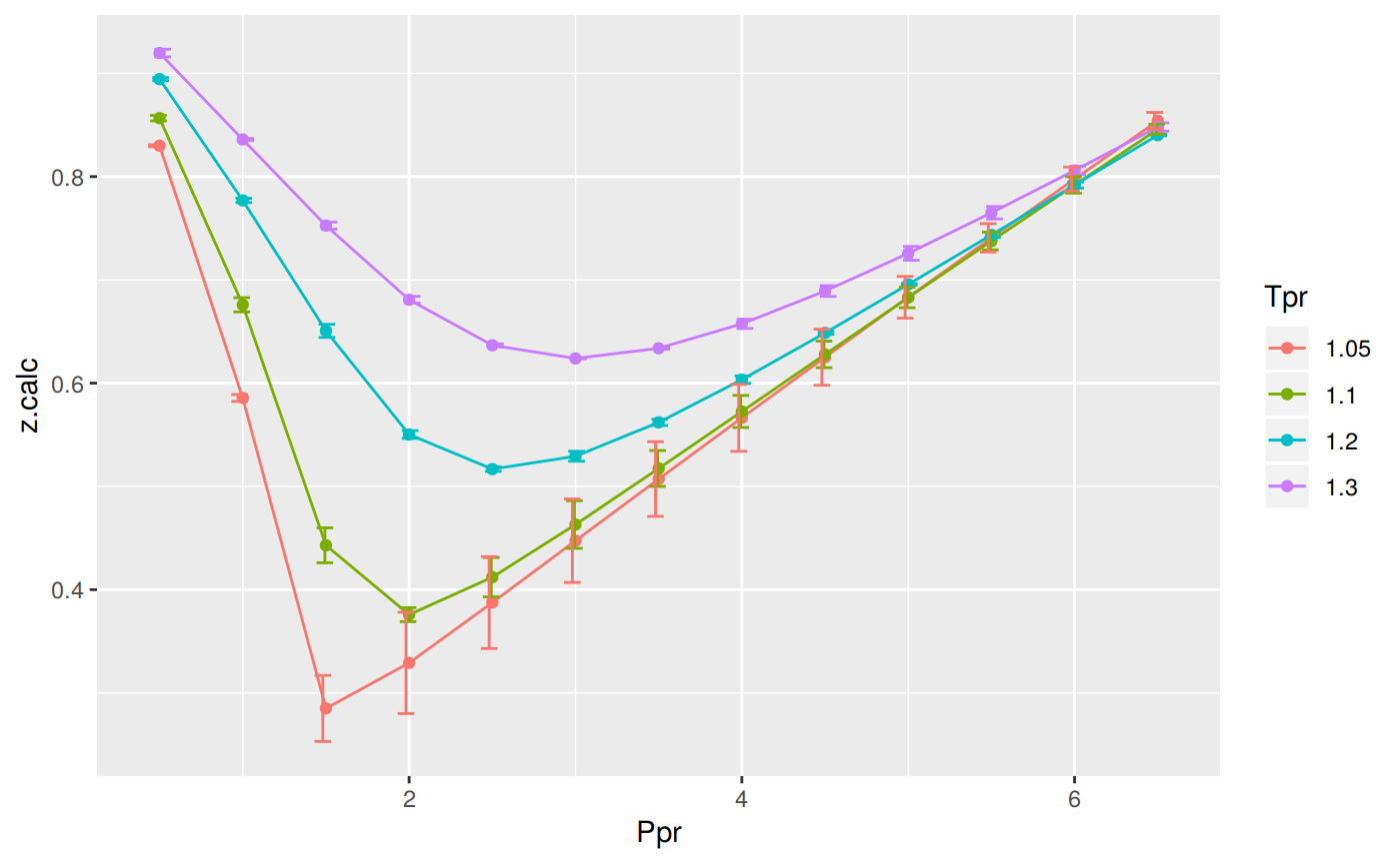

# A tibble: 52 x 5
   Tpr     Ppr z.chart z.calc       dif
   <chr> <dbl>   <dbl>  <dbl>     <dbl>
 1 1.05    0.5   0.829  0.830 -0.000976
 2 1.1     0.5   0.854  0.857 -0.00264 
 3 1.2     0.5   0.893  0.894 -0.00146 
 4 1.3     0.5   0.916  0.920 -0.00372 
 5 1.05    1     0.589  0.586  0.00333 
 6 1.1     1     0.669  0.676 -0.00689 
 7 1.2     1     0.779  0.777  0.00205 
 8 1.3     1     0.835  0.836 -0.000989
 9 1.05    1.5   0.253  0.285 -0.0320  
10 1.1     1.5   0.426  0.443 -0.0169  
# … with 42 more rows

We observe that with Dranchuk-Purvis-Robinson there are still errors or differences between the z values in the Standing-Katz chart and the values obtained from the correlation but they are not so bad as in the HY correlation.

Analysis at the lowest Tpr

This is the isotherm where we see the greatest error.

library(zFactor)

sk_corr_3 <- sk_corr_2[sk_corr_2$Tpr==1.05,]
sk_corr_3

p <- ggplot(sk_corr_3, aes(x=Ppr, y=z.calc, group=Tpr, color=Tpr)) +
    geom_line() +
    geom_point() +
    geom_errorbar(aes(ymin=z.calc-dif, ymax=z.calc+dif), width=.2,
                  position=position_dodge(0.05))
print(p)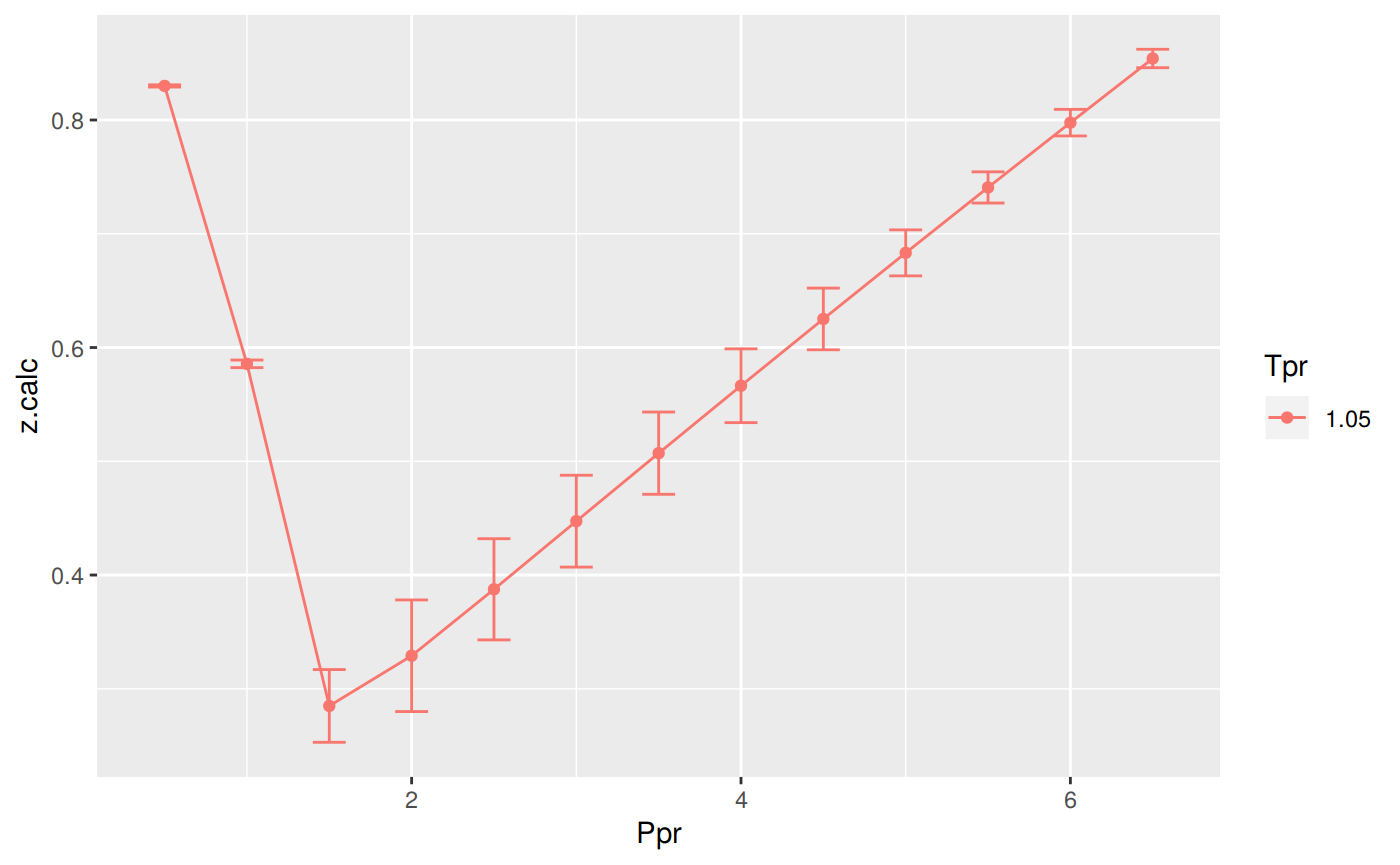

    Tpr Ppr z.chart    z.calc           dif
1  1.05 0.5   0.829 0.8299757 -0.0009756528
5  1.05 1.0   0.589 0.5856680  0.0033320375
9  1.05 1.5   0.253 0.2849670 -0.0319670358
13 1.05 2.0   0.280 0.3290685 -0.0490685223
17 1.05 2.5   0.343 0.3874732 -0.0444731970
21 1.05 3.0   0.407 0.4473627 -0.0403627209
25 1.05 3.5   0.471 0.5071451 -0.0361451067
29 1.05 4.0   0.534 0.5664346 -0.0324345927
33 1.05 4.5   0.598 0.6251306 -0.0271306123
37 1.05 5.0   0.663 0.6832213 -0.0202213318
41 1.05 5.5   0.727 0.7407256 -0.0137256422
45 1.05 6.0   0.786 0.7976728 -0.0116727857
49 1.05 6.5   0.846 0.8540945 -0.0080944856

Analyzing performance of the DPR correlation for all the Tpr curves

In this last example, we compare the values of z at all the isotherms. We use the function getStandingKatzTpr to obtain all the isotherms or Tpr curves in the Standing-Katz chart that have been digitized. The next function createTidyFromMatrix calculate z using the correlation and prepares a tidy dataset ready to plot.

library(ggplot2)
library(tibble)

# get all `lp` Tpr curves
tpr_all <- getStandingKatzTpr(pprRange = "lp")
ppr <- c(0.5, 1.5, 2.5, 3.5, 4.5, 5.5, 6.5) 

sk_corr_all <- createTidyFromMatrix(ppr, tpr_all, correlation = "DPR")
as_tibble(sk_corr_all)

p <- ggplot(sk_corr_all, aes(x=Ppr, y=z.calc, group=Tpr, color=Tpr)) +
    geom_line() +
    geom_point() +
    geom_errorbar(aes(ymin=z.calc-dif, ymax=z.calc+dif), width=.4,
                  position=position_dodge(0.05))
print(p)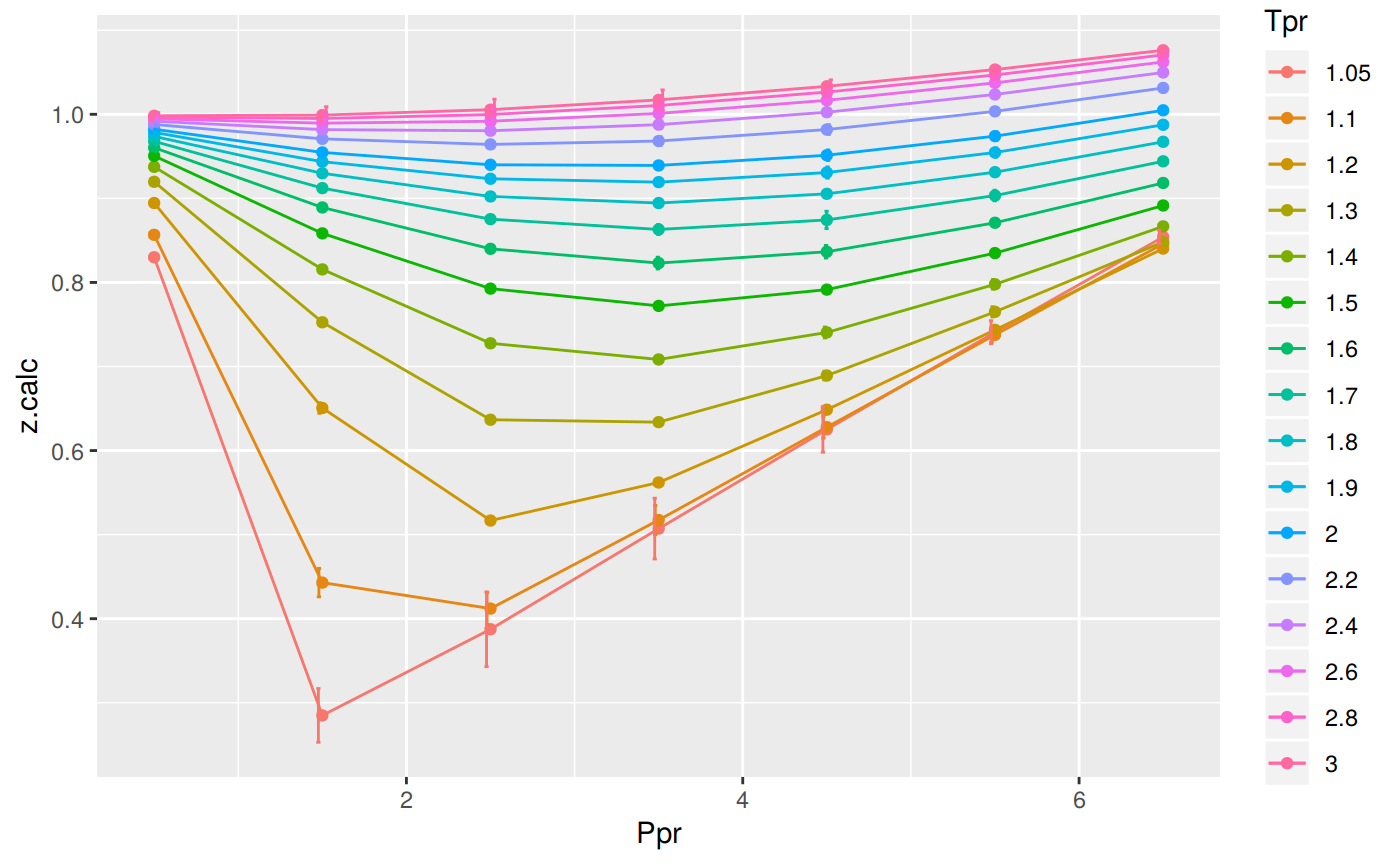

# A tibble: 112 x 5
   Tpr     Ppr z.chart z.calc       dif
   <chr> <dbl>   <dbl>  <dbl>     <dbl>
 1 1.05    0.5   0.829  0.830 -0.000976
 2 1.1     0.5   0.854  0.857 -0.00264 
 3 1.2     0.5   0.893  0.894 -0.00146 
 4 1.3     0.5   0.916  0.920 -0.00372 
 5 1.4     0.5   0.936  0.937 -0.00149 
 6 1.5     0.5   0.948  0.950 -0.00248 
 7 1.6     0.5   0.959  0.960 -0.00126 
 8 1.7     0.5   0.968  0.968  0.000216
 9 1.8     0.5   0.974  0.974  0.000310
10 1.9     0.5   0.978  0.978 -0.000398
# … with 102 more rows

The greatest errors are localized in two of the Tpr curves: at 1.05 and 1.1.

Range of applicability of the correlation

# MSE: Mean Squared Error
# RMSE: Root Mean Squared Error
# RSS: residual sum of square
# ARE:  Average Relative Error, %
# AARE: Average Absolute Relative Error, %
library(dplyr)
grouped <- group_by(sk_corr_all, Tpr, Ppr)

smry_tpr_ppr <- summarise(grouped, 
          RMSE= sqrt(mean((z.chart-z.calc)^2)), 
          MPE = sum((z.calc - z.chart) / z.chart) * 100 / n(),
          MAPE = sum(abs((z.calc - z.chart) / z.chart)) * 100 / n(), 
          MSE = sum((z.calc - z.chart)^2) / n(), 
          RSS = sum((z.calc - z.chart)^2),
          MAE = sum(abs(z.calc - z.chart)) / n(),
          RMLSE = sqrt(1/n()*sum((log(z.calc +1)-log(z.chart +1))^2))
          )

ggplot(smry_tpr_ppr, aes(Ppr, Tpr)) + 
    geom_tile(data=smry_tpr_ppr, aes(fill=MAPE), color="white") +
    scale_fill_gradient2(low="blue", high="red", mid="yellow", na.value = "pink",
                         midpoint=12.5, limit=c(0, 25), name="MAPE") + 
    theme(axis.text.x = element_text(angle=45, vjust=1, size=11, hjust=1)) + 
    coord_equal() +
    ggtitle("Dranchuk-Purvis-Robinson", subtitle = "DPR")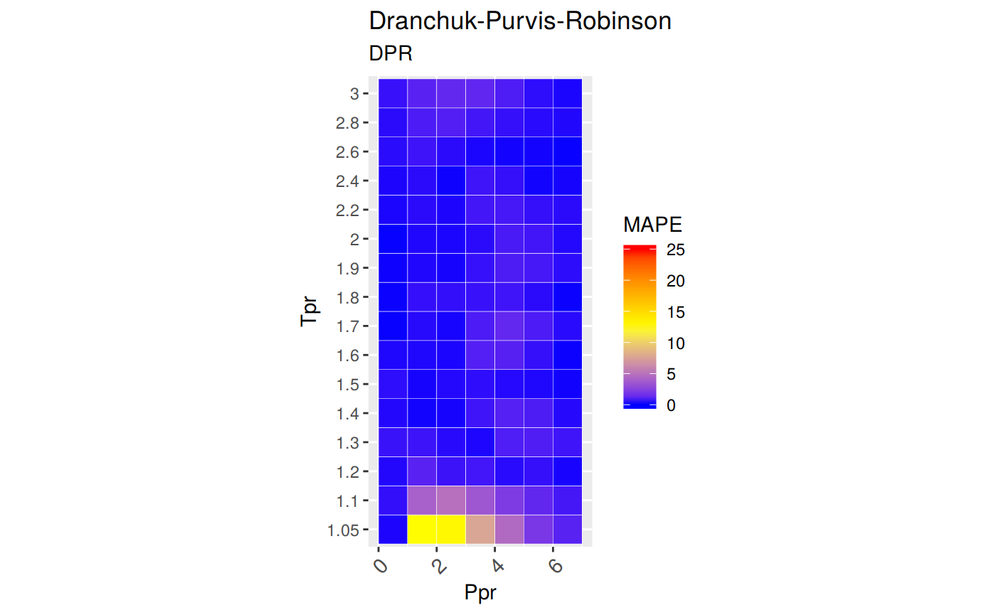

The greatest errors are localized in two of the Tpr curves: 1.05 and barely at 1.1

Plotting the Tpr and Ppr values that show more error

library(dplyr)

sk_corr_all %>%
    filter(Tpr %in% c("1.05", "1.1")) %>%
    ggplot(aes(x = z.chart, y=z.calc, group = Tpr, color = Tpr)) +
    geom_point(size = 3) +
    geom_line(aes(x = z.chart, y = z.chart), color = "black") +
    facet_grid(. ~ Tpr) +
    geom_errorbar(aes(ymin=z.calc-abs(dif), ymax=z.calc+abs(dif)), 
                  position=position_dodge(0.5))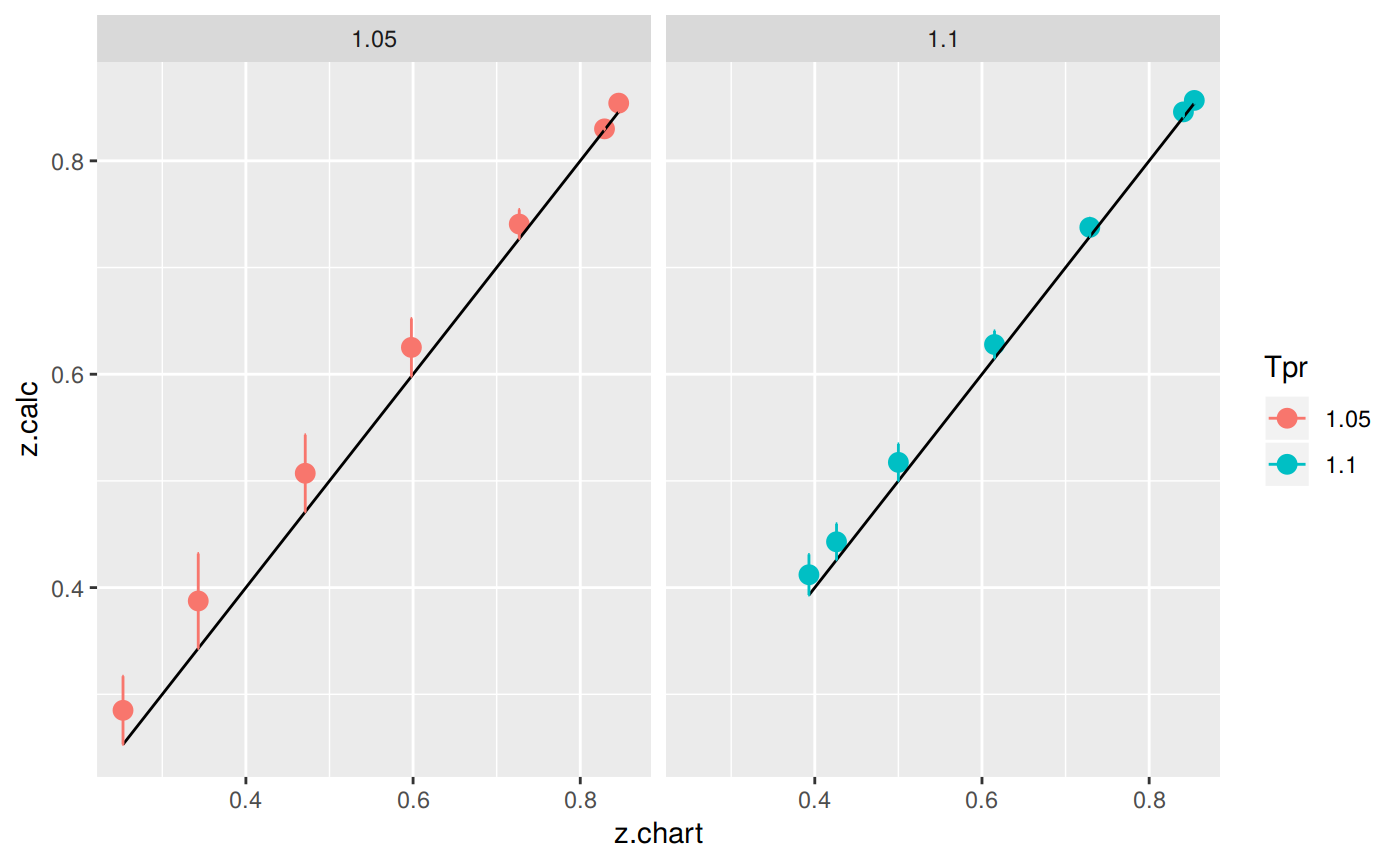

Looking numerically at the errors

Finally, the dataframe with the calculated errors between the z from the correlation and the z read from the chart:

as_tibble(smry_tpr_ppr)

# A tibble: 112 x 9
   Tpr     Ppr     RMSE    MPE   MAPE        MSE        RSS     MAE   RMLSE
   <chr> <dbl>    <dbl>  <dbl>  <dbl>      <dbl>      <dbl>   <dbl>   <dbl>
 1 1.05    0.5 0.000976  0.118  0.118    9.52e-7    9.52e-7 9.76e-4 5.33e-4
 2 1.05    1.5 0.0320   12.6   12.6      1.02e-3    1.02e-3 3.20e-2 2.52e-2
 3 1.05    2.5 0.0445   13.0   13.0      1.98e-3    1.98e-3 4.45e-2 3.26e-2
 4 1.05    3.5 0.0361    7.67   7.67     1.31e-3    1.31e-3 3.61e-2 2.43e-2
 5 1.05    4.5 0.0271    4.54   4.54     7.36e-4    7.36e-4 2.71e-2 1.68e-2
 6 1.05    5.5 0.0137    1.89   1.89     1.88e-4    1.88e-4 1.37e-2 7.92e-3
 7 1.05    6.5 0.00809   0.957  0.957    6.55e-5    6.55e-5 8.09e-3 4.38e-3
 8 1.1     0.5 0.00264   0.309  0.309    6.95e-6    6.95e-6 2.64e-3 1.42e-3
 9 1.1     1.5 0.0169    3.98   3.98     2.87e-4    2.87e-4 1.69e-2 1.18e-2
10 1.1     2.5 0.0191    4.85   4.85     3.63e-4    3.63e-4 1.91e-2 1.36e-2
# … with 102 more rows

References

Dranchuk, Peter M, RA Purvis, DB Robinson, and others. 1973. “Computer Calculation of Natural Gas Compressibility Factors Using the Standing and Katz Correlation.” In Annual Technical Meeting, edited by unknown. Petroleum Society of Canada. https://doi.org/10.2118/73-112.