Dranchuk-AbouKassem correlation

2019-08-01

The DAK correlation

The work by P.M. Dranchuk and J.H. Abou-Kassem was looking to examine z outside the regions established by the Standing-Katz chart. They used as a basis the generalized Starling equation of state. They provided the code in FORTRAN. See (Dranchuk and Abou-Kassem 1975)

Get z at selected Ppr and Tpr

Use the the correlation to calculate z and from Standing-Katz chart obtain z a digitized point at the given Tpr and Ppr.

# get a z value
library(zFactor)

ppr <- 1.5
tpr <- 2.0

z.calc <- z.DranchukAbuKassem(pres.pr = ppr, temp.pr = tpr)

# get a z value from the SK chart at the same Ppr and Tpr

z.chart <- getStandingKatzMatrix(tpr_vector = tpr, 
                      pprRange = "lp")[1, as.character(ppr)]


# calculate the APE
ape <- abs((z.calc - z.chart) / z.chart) * 100

df <- as.data.frame(list(Ppr = ppr,  z.calc =z.calc, z.chart = z.chart, ape=ape))
rownames(df) <- tpr
df
# HY = 0.9580002; # DAK = 0.9551087

  Ppr    z.calc z.chart        ape
2 1.5 0.9551087   0.956 0.09322868

Get z at selected Ppr and Tpr=1.1

From the Standing-Katz chart we read z at a digitized point:

library(zFactor)

ppr <- 1.5
tpr <- 1.1

z.calc <- z.DranchukAbuKassem(pres.pr = ppr, temp.pr = tpr)

# From the Standing-Katz chart we obtain a digitized point:
z.chart <- getStandingKatzMatrix(tpr_vector = tpr, 
                      pprRange = "lp")[1, as.character(ppr)]

# calculate the APE (Average Percentage Error)
ape <- abs((z.calc - z.chart) / z.chart) * 100

df <- as.data.frame(list(Ppr = ppr,  z.calc =z.calc, z.chart = z.chart, ape=ape))
rownames(df) <- tpr
df

    Ppr    z.calc z.chart     ape
1.1 1.5 0.4463987   0.426 4.78842

At lower Tpr we can see that there is some difference between the values of z from the DAK calculation and the z value read from the Standing-Katz chart. See the APE.

Get values of z for combinations of Ppr and Tpr

In this example we provide vectors instead of a single point. With the same ppr and tpr vectors that we use for the correlation, we do the same for the Standing-Katz chart. We want to compare both and find the absolute percentage error or APE.

# test DAK with 1st-derivative using the values from paper 
ppr <- c(0.5, 1.5, 2.5, 3.5, 4.5, 5.5, 6.5) 
tpr <- c(1.05, 1.1, 1.7, 2) 

# calculate using the correlation
z.calc <- z.DranchukAbuKassem(ppr, tpr)

# With the same ppr and tpr vector, we do the same for the Standing-Katz chart
z.chart <- getStandingKatzMatrix(ppr_vector = ppr, tpr_vector = tpr)
ape <- abs((z.calc - z.chart) / z.chart) * 100

# calculate the APE
cat("z.correlation \n"); print(z.calc)
cat("\n z.chart \n"); print(z.chart)
cat("\n APE \n"); print(ape)

z.correlation 
           0.5       1.5       2.5       3.5       4.5       5.5       6.5
1.05 0.8300683 0.2837318 0.3868282 0.5063005 0.6239783 0.7392097 0.8521762
1.1  0.8570452 0.4463987 0.4125200 0.5178068 0.6281858 0.7378206 0.8458725
1.7  0.9681353 0.9128087 0.8753784 0.8619509 0.8721085 0.9003962 0.9409634
2    0.9824731 0.9551087 0.9400752 0.9385273 0.9497137 0.9715388 1.0015560

 z.chart 
       0.5   1.5   2.5   3.5   4.5   5.5   6.5
1.05 0.829 0.253 0.343 0.471 0.598 0.727 0.846
1.10 0.854 0.426 0.393 0.500 0.615 0.729 0.841
1.70 0.968 0.914 0.876 0.857 0.864 0.897 0.942
2.00 0.982 0.956 0.941 0.937 0.945 0.969 1.003

 APE 
            0.5         1.5         2.5       3.5       4.5       5.5
1.05 0.12887088 12.14694898 12.77790878 7.4947969 4.3441895 1.6794701
1.1  0.35658638  4.78841969  4.96692005 3.5613696 2.1440308 1.2099607
1.7  0.01397555  0.13033558  0.07096218 0.5776995 0.9384799 0.3786176
2    0.04818209  0.09322868  0.09827500 0.1629967 0.4988064 0.2620070
           6.5
1.05 0.7300441
1.1  0.5793746
1.7  0.1100436
2    0.1439679

You can see errors of 12.15% and 12.78% in the isotherm Tpr=1.05 at Ppr 0.5 and 2.5. Other errors, greater than one, can also be found at the isotherm Tpr=1.1: 4.97%. Then, the rest of the Tpr curves are fine.

Analyze the error at the isotherms

Applying the function summary over the transpose of the matrix:

sum_t_ape <- summary(t(ape))
sum_t_ape

      1.05              1.1              1.7                2          
 Min.   : 0.1289   Min.   :0.3566   Min.   :0.01398   Min.   :0.04818  
 1st Qu.: 1.2048   1st Qu.:0.8947   1st Qu.:0.09050   1st Qu.:0.09575  
 Median : 4.3442   Median :2.1440   Median :0.13034   Median :0.14397  
 Mean   : 5.6146   Mean   :2.5152   Mean   :0.31716   Mean   :0.18678  
 3rd Qu.: 9.8209   3rd Qu.:4.1749   3rd Qu.:0.47816   3rd Qu.:0.21250  
 Max.   :12.7779   Max.   :4.9669   Max.   :0.93848   Max.   :0.49881  

We can see that the errors in z are considerable with a Min. : 0.1289 % and Max. :12.7779 % for Tpr=1.05, and a Min. :0.3566 % and Max. :4.9669 % for Tpr=1.10. We will explore later a comparative tile chart where we confirm these early calculations.

Analyze the error for greater values of Tpr

library(zFactor)
# enter vectors for Tpr and Ppr
tpr2 <- c(1.2, 1.3, 1.5, 2.0, 3.0) 
ppr2 <- c(0.5, 1.5, 2.5, 3.5, 4.5, 5.5) 

# get z values from the SK chart
z.chart <- getStandingKatzMatrix(ppr_vector = ppr2, tpr_vector = tpr2, pprRange = "lp")

# We do the same with the HY correlation:
# calculate z values at lower values of Tpr
z.calc <- z.DranchukAbuKassem(pres.pr = ppr2, temp.pr = tpr2) 
ape <- abs((z.calc - z.chart) / z.chart) * 100

# calculate the APE
cat("z.correlation \n"); print(z.calc)
cat("\n z.chart \n"); print(z.chart)
cat("\n APE \n"); print(ape)

z.correlation 
          0.5       1.5       2.5       3.5       4.5       5.5
1.2 0.8950631 0.6532419 0.5180675 0.5631805 0.6501377 0.7453363
1.3 0.9203019 0.7543694 0.6377871 0.6339357 0.6898314 0.7663247
1.5 0.9509373 0.8593144 0.7929993 0.7710525 0.7896224 0.8331893
2   0.9824731 0.9551087 0.9400752 0.9385273 0.9497137 0.9715388
3   0.9984498 0.9995529 1.0061111 1.0176846 1.0336417 1.0532809

 z.chart 
       0.5   1.5   2.5   3.5   4.5   5.5
1.20 0.893 0.657 0.519 0.565 0.650 0.741
1.30 0.916 0.756 0.638 0.633 0.684 0.759
1.50 0.948 0.859 0.794 0.770 0.790 0.836
2.00 0.982 0.956 0.941 0.937 0.945 0.969
3.00 1.002 1.009 1.018 1.029 1.041 1.056

 APE 
           0.5        1.5        2.5       3.5        4.5       5.5
1.2 0.23103290 0.57200352 0.17966969 0.3220337 0.02117873 0.5851899
1.3 0.46964046 0.21568687 0.03336463 0.1478274 0.85254906 0.9650399
1.5 0.30984425 0.03659844 0.12603050 0.1366918 0.04779169 0.3362070
2   0.04818209 0.09322868 0.09827500 0.1629967 0.49880636 0.2620070
3   0.35430932 0.93627979 1.16787124 1.0996524 0.70685120 0.2574863

We observe that at Tpr above or equal to 1.2 the DAK correlation behaves very well.

Analyze the error at the isotherms

Applying the function summary over the transpose of the matrix to observe the error of the correlation at each isotherm.

sum_t_ape <- summary(t(ape))
sum_t_ape
 # Hall-Yarborough
 #      1.2               1.3              1.5               2         
 # Min.   :0.05224   Min.   :0.1105   Min.   :0.1021   Min.   :0.0809  
 # 1st Qu.:0.09039   1st Qu.:0.2080   1st Qu.:0.1623   1st Qu.:0.1814  
 # Median :0.28057   Median :0.3181   Median :0.1892   Median :0.1975  
 # Mean   :0.30122   Mean   :0.3899   Mean   :0.2597   Mean   :0.2284  
 # 3rd Qu.:0.51710   3rd Qu.:0.5355   3rd Qu.:0.3533   3rd Qu.:0.2627  
 # Max.   :0.57098   Max.   :0.8131   Max.   :0.5162   Max.   :0.4338  
 #       3          
 # Min.   :0.09128  
 # 1st Qu.:0.17466  
 # Median :0.35252  
 # Mean   :0.34820  
 # 3rd Qu.:0.52184  
 # Max.   :0.59923  

      1.2               1.3               1.5                2          
 Min.   :0.02118   Min.   :0.03336   Min.   :0.03660   Min.   :0.04818  
 1st Qu.:0.19251   1st Qu.:0.16479   1st Qu.:0.06735   1st Qu.:0.09449  
 Median :0.27653   Median :0.34266   Median :0.13136   Median :0.13064  
 Mean   :0.31852   Mean   :0.44735   Mean   :0.16553   Mean   :0.19392  
 3rd Qu.:0.50951   3rd Qu.:0.75682   3rd Qu.:0.26656   3rd Qu.:0.23725  
 Max.   :0.58519   Max.   :0.96504   Max.   :0.33621   Max.   :0.49881  
       3         
 Min.   :0.2575  
 1st Qu.:0.4424  
 Median :0.8216  
 Mean   :0.7537  
 3rd Qu.:1.0588  
 Max.   :1.1679  

We can see that the errors in z with DAK are far lower than Hall-Yarborough with a Min. :0.02118 % and Max. :0.58519 % for Tpr=1.2, and a Min. :0.03336 % and Max. :0.96504 % for Tpr=1.3.

Prepare to plot SK vs DAK correlation

The error bars represent the difference between the calculated values by the Dranchuk-AbouKassem corrrelation and teh values of z read from the Standing-Katz chart.

library(zFactor)
library(tibble)
library(ggplot2)

tpr2 <- c(1.05, 1.1, 1.2, 1.3) 
ppr2 <- c(0.5, 1.0, 1.5, 2, 2.5, 3.0, 3.5, 4.0, 4.5, 5.0, 5.5, 6.0, 6.5) 

sk_dak_2 <- createTidyFromMatrix(ppr2, tpr2, correlation = "DAK")
as_tibble(sk_dak_2)


p <- ggplot(sk_dak_2, aes(x=Ppr, y=z.calc, group=Tpr, color=Tpr)) +
    geom_line() +
    geom_point() +
    geom_errorbar(aes(ymin=z.calc-dif, ymax=z.calc+dif), width=.4,
                  position=position_dodge(0.05))
print(p)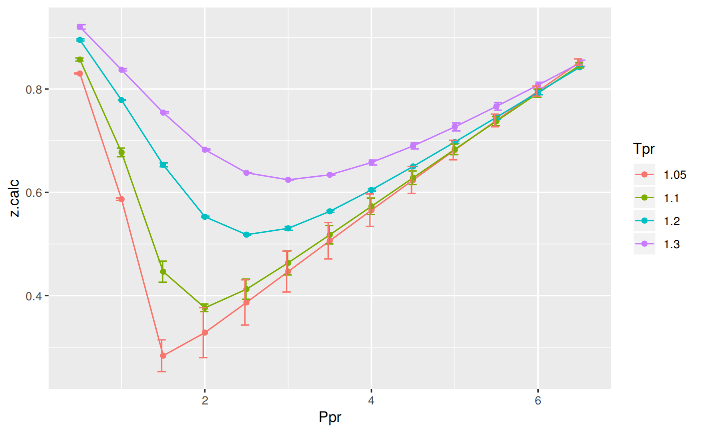

# A tibble: 52 x 5
   Tpr     Ppr z.chart z.calc       dif
   <chr> <dbl>   <dbl>  <dbl>     <dbl>
 1 1.05    0.5   0.829  0.830 -0.00107 
 2 1.1     0.5   0.854  0.857 -0.00305 
 3 1.2     0.5   0.893  0.895 -0.00206 
 4 1.3     0.5   0.916  0.920 -0.00430 
 5 1.05    1     0.589  0.587  0.00232 
 6 1.1     1     0.669  0.677 -0.00837 
 7 1.2     1     0.779  0.778  0.000578
 8 1.3     1     0.835  0.837 -0.00221 
 9 1.05    1.5   0.253  0.284 -0.0307  
10 1.1     1.5   0.426  0.446 -0.0204  
# … with 42 more rows

We observe that with Dranchuk-AbouKassem there are still errors or differences between the z values in the Standing-Katz chart and the values obtained from the correlation but they are not as bad as in the HY correlation.

Analysis at the lowest Tpr

This is the isotherm where we see the greatest error.

library(zFactor)

sk_dak_3 <- sk_dak_2[sk_dak_2$Tpr==1.05,]
sk_dak_3

p <- ggplot(sk_dak_3, aes(x=Ppr, y=z.calc, group=Tpr, color=Tpr)) +
    geom_line() +
    geom_point() +
    geom_errorbar(aes(ymin=z.calc-dif, ymax=z.calc+dif), width=.2,
                  position=position_dodge(0.05))
print(p)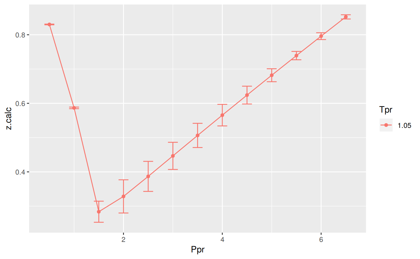

    Tpr Ppr z.chart    z.calc          dif
1  1.05 0.5   0.829 0.8300683 -0.001068340
5  1.05 1.0   0.589 0.5866751  0.002324861
9  1.05 1.5   0.253 0.2837318 -0.030731781
13 1.05 2.0   0.280 0.3284040 -0.048404016
17 1.05 2.5   0.343 0.3868282 -0.043828227
21 1.05 3.0   0.407 0.4466387 -0.039638654
25 1.05 3.5   0.471 0.5063005 -0.035300493
29 1.05 4.0   0.534 0.5654448 -0.031444815
33 1.05 4.5   0.598 0.6239783 -0.025978253
37 1.05 5.0   0.663 0.6818928 -0.018892813
41 1.05 5.5   0.727 0.7392097 -0.012209748
45 1.05 6.0   0.786 0.7959599 -0.009959903
49 1.05 6.5   0.846 0.8521762 -0.006176173

Analyzing performance of the DAK correlation for all the Tpr curves

In this last example, we compare the values of z at all the isotherms. We use the function getCurvesDigitized to obtain all the isotherms or Tpr curves in the Standing-Katz chart that have been digitized. The next function createTidyFromMatrix calculate z using the correlation and prepares a tidy dataset ready to plot.

library(ggplot2)
library(tibble)

# get all `lp` Tpr curves
tpr_all <- getStandingKatzTpr(pprRange = "lp")
ppr <- c(0.5, 1.5, 2.5, 3.5, 4.5, 5.5, 6.5) 
sk_corr_all <- createTidyFromMatrix(ppr, tpr_all, correlation = "DAK")
as_tibble(sk_corr_all)

p <- ggplot(sk_corr_all, aes(x=Ppr, y=z.calc, group=Tpr, color=Tpr)) +
    geom_line() +
    geom_point() +
    geom_errorbar(aes(ymin=z.calc-dif, ymax=z.calc+dif), width=.4,
                  position=position_dodge(0.05))
print(p)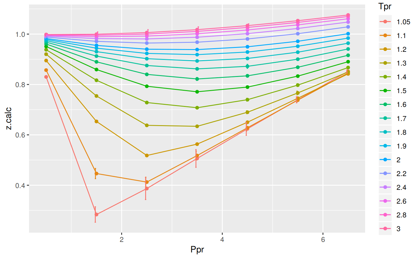

# A tibble: 112 x 5
   Tpr     Ppr z.chart z.calc         dif
   <chr> <dbl>   <dbl>  <dbl>       <dbl>
 1 1.05    0.5   0.829  0.830 -0.00107   
 2 1.1     0.5   0.854  0.857 -0.00305   
 3 1.2     0.5   0.893  0.895 -0.00206   
 4 1.3     0.5   0.916  0.920 -0.00430   
 5 1.4     0.5   0.936  0.938 -0.00201   
 6 1.5     0.5   0.948  0.951 -0.00294   
 7 1.6     0.5   0.959  0.961 -0.00165   
 8 1.7     0.5   0.968  0.968 -0.000135  
 9 1.8     0.5   0.974  0.974 -0.00000593
10 1.9     0.5   0.978  0.979 -0.000688  
# … with 102 more rows

The greatest errors are localized in two of the Tpr curves: at 1.05 and 1.1.

Range of applicability of the correlation

# MSE: Mean Squared Error
# RMSE: Root Mean Squared Error
# RSS: residual sum of square
# ARE:  Average Relative Error, %
# AARE: Average Absolute Relative Error, %
library(dplyr)
grouped <- group_by(sk_corr_all, Tpr, Ppr)

smry_tpr_ppr <- summarise(grouped, 
          RMSE= sqrt(mean((z.chart-z.calc)^2)), 
          MPE = sum((z.calc - z.chart) / z.chart) * 100 / n(),
          MAPE = sum(abs((z.calc - z.chart) / z.chart)) * 100 / n(), 
          MSE = sum((z.calc - z.chart)^2) / n(), 
          RSS = sum((z.calc - z.chart)^2),
          MAE = sum(abs(z.calc - z.chart)) / n(),
          RMLSE = sqrt(1/n()*sum((log(z.calc +1)-log(z.chart +1))^2))
          )

ggplot(smry_tpr_ppr, aes(Ppr, Tpr)) + 
    geom_tile(data=smry_tpr_ppr, aes(fill=MAPE), color="white") +
    scale_fill_gradient2(low="blue", high="red", mid="yellow", na.value = "pink",
                         midpoint=12.5, limit=c(0, 25), name="MAPE") + 
    theme(axis.text.x = element_text(angle=45, vjust=1, size=11, hjust=1)) + 
    coord_equal() +
    ggtitle("Dranchuk-AbouKassem", subtitle = "DAK")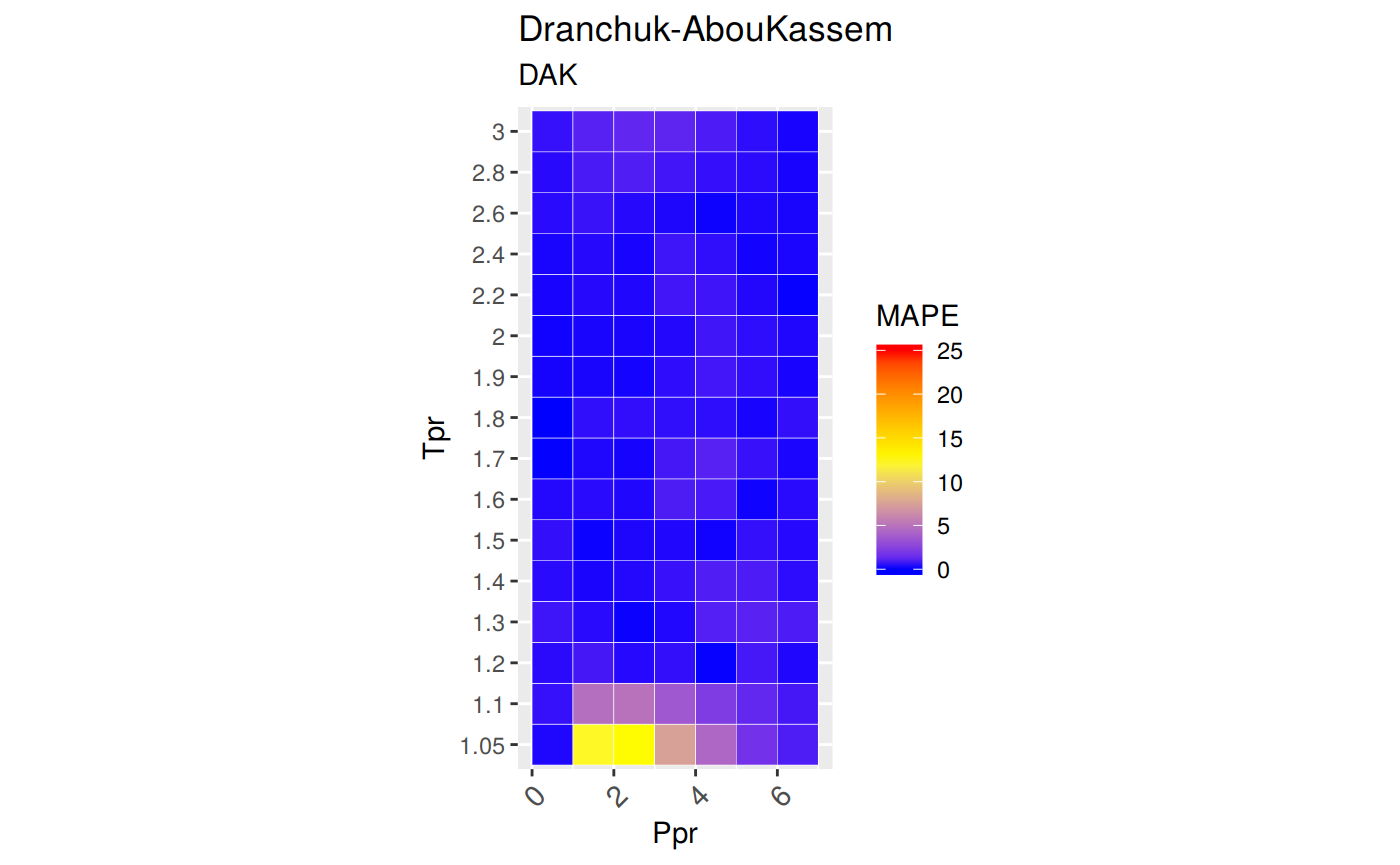

The greatest errors are localized in two of the Tpr curves: 1.05 and barely at 1.1. But the errors are smaller than that we saw in the HY plot.

Plotting the Tpr and Ppr values that show more error

The MAPE (mean average percentage error) gradient bar indicates that the more red the square is, the more error there is.

library(dplyr)

sk_corr_all %>%
    filter(Tpr %in% c("1.05", "1.1")) %>%
    ggplot(aes(x = z.chart, y=z.calc, group = Tpr, color = Tpr)) +
    geom_point(size = 3) +
    geom_line(aes(x = z.chart, y = z.chart), color = "black") +
    facet_grid(. ~ Tpr) +
    geom_errorbar(aes(ymin=z.calc-abs(dif), ymax=z.calc+abs(dif)), 
                  position=position_dodge(0.5))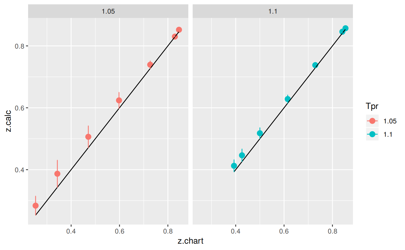

Looking numerically at the errors

Finally, the dataframe with the calculated errors between the z from the correlation and the z read from the chart:

as_tibble(smry_tpr_ppr)

# A tibble: 112 x 9
   Tpr     Ppr    RMSE    MPE   MAPE        MSE        RSS     MAE    RMLSE
   <chr> <dbl>   <dbl>  <dbl>  <dbl>      <dbl>      <dbl>   <dbl>    <dbl>
 1 1.05    0.5 0.00107  0.129  0.129 0.00000114 0.00000114 0.00107 0.000584
 2 1.05    1.5 0.0307  12.1   12.1   0.000944   0.000944   0.0307  0.0242  
 3 1.05    2.5 0.0438  12.8   12.8   0.00192    0.00192    0.0438  0.0321  
 4 1.05    3.5 0.0353   7.49   7.49  0.00125    0.00125    0.0353  0.0237  
 5 1.05    4.5 0.0260   4.34   4.34  0.000675   0.000675   0.0260  0.0161  
 6 1.05    5.5 0.0122   1.68   1.68  0.000149   0.000149   0.0122  0.00705 
 7 1.05    6.5 0.00618  0.730  0.730 0.0000381  0.0000381  0.00618 0.00334 
 8 1.1     0.5 0.00305  0.357  0.357 0.00000927 0.00000927 0.00305 0.00164 
 9 1.1     1.5 0.0204   4.79   4.79  0.000416   0.000416   0.0204  0.0142  
10 1.1     2.5 0.0195   4.97   4.97  0.000381   0.000381   0.0195  0.0139  
# … with 102 more rows

References

Dranchuk, P. M., and H. Abou-Kassem. 1975. “Calculation of Z Factors for Natural Gases Using Equations of State.” Journal of Canadian Petroleum Technology, July. Petroleum Society of Canada. https://doi.org/10.2118/75-03-03.