Hall-Yarborough correlation

2019-08-01

The Hall-Yarborough correlation

Kenneth Hall and Lyman Yarborough used the hard-sphere equation as the basis for the equation of state. They tested the correlation with 12 reservoir gas reservoir systems up to Ppr as high as 20.5. The Standing-Katz chart only extends to Ppr=15. At that moment the Standing-Katz chart had 30 years of existance. See (Hall and Yarborough 1973).

Get z at selected Ppr and Tpr=2.0

Use the the corelation to calculate z. From the Standing-Katz chart we obtain a digitized point at the given Tpr and Ppr.

# get a z value using HY
library(zFactor)

ppr <- 1.5
tpr <- 2.0

z.calc <- z.HallYarborough(pres.pr = ppr, temp.pr = tpr)

# get a z value from the SK chart at the same Ppr and Tpr
z.chart <- getStandingKatzMatrix(tpr_vector = tpr, 
                      pprRange = "lp")[1, as.character(ppr)]

# calculate the APE (Average Percentage Error)
ape <- abs((z.calc - z.chart) / z.chart) * 100

df <- as.data.frame(list(Ppr = ppr,  z.calc =z.calc, z.chart = z.chart, ape=ape))
rownames(df) <- tpr
df

  Ppr    z.calc z.chart      ape
2 1.5 0.9580002   0.956 0.209229

Get z at selected Ppr and Tpr = 1.1

From the Standing-Katz chart we obtain a digitized point:

library(zFactor)
ppr <- 1.5
tpr <- 1.1

z.calc <- z.HallYarborough(pres.pr = ppr, temp.pr = tpr)

# From the Standing-Katz chart we obtain a digitized point:
z.chart <- getStandingKatzMatrix(tpr_vector = tpr, 
                      pprRange = "lp")[1, as.character(ppr)]

# calculate the APE
ape <- abs((z.calc - z.chart) / z.chart) * 100

df <- as.data.frame(list(Ppr = ppr,  z.calc =z.calc, z.chart = z.chart, ape=ape))
rownames(df) <- tpr
df

    Ppr    z.calc z.chart      ape
1.1 1.5 0.4732393   0.426 11.08903

We see here a noticeable difference between the values of z from the HY correlation and the value read from the Standing-Katz chart. This is expected at these low pressures and temperatures. This area is a challenge for all of the correlations as well.

Get values of z for combinations of Ppr and Tpr

In this example we provide vectors instead of a single point. With the same ppr and tpr vectors that we use for the correlation, we do the same for the Standing-Katz chart. We want to compare both and find the absolute percentage error.

library(zFactor)

ppr <- c(0.5, 1.5, 2.5, 3.5, 4.5, 5.5, 6.5) 
tpr <- c(1.05, 1.1, 1.7, 2) 

# calculate using the correlation
z.calc <- z.HallYarborough(ppr, tpr)

# With the same ppr and tpr vector, we do the same for the Standing-Katz chart
z.chart <- getStandingKatzMatrix(ppr_vector = ppr, tpr_vector = tpr)
ape <- abs((z.calc - z.chart) / z.chart) * 100

# calculate the APE
cat("z.correlation \n"); print(z.calc)
cat("\n z.chart \n"); print(z.chart)
cat("\n APE \n"); print(ape)

z.correlation 
           0.5       1.5       2.5       3.5       4.5       5.5       6.5
1.05 0.8324659 0.3098781 0.3844710 0.4996188 0.6150882 0.7291019 0.8415294
1.1  0.8565046 0.4732393 0.4138513 0.5136995 0.6220391 0.7307972 0.8386698
1.7  0.9682547 0.9134862 0.8756412 0.8605668 0.8694525 0.8978885 0.9396353
2    0.9838234 0.9580002 0.9426939 0.9396286 0.9490995 0.9697839 0.9994317

 z.chart 
       0.5   1.5   2.5   3.5   4.5   5.5   6.5
1.05 0.829 0.253 0.343 0.471 0.598 0.727 0.846
1.10 0.854 0.426 0.393 0.500 0.615 0.729 0.841
1.70 0.968 0.914 0.876 0.857 0.864 0.897 0.942
2.00 0.982 0.956 0.941 0.937 0.945 0.969 1.003

 APE 
            0.5         1.5         2.5       3.5       4.5        5.5
1.05 0.41807702 22.48144801 12.09066991 6.0761856 2.8575603 0.28912295
1.1  0.29327707 11.08903030  5.30568143 2.7398940 1.1445758 0.24652442
1.7  0.02631234  0.05621824  0.04096114 0.4162014 0.6310709 0.09904802
2    0.18568379  0.20922900  0.18000605 0.2805309 0.4338140 0.08089785
           6.5
1.05 0.5284438
1.1  0.2770741
1.7  0.2510320
2    0.3557593

You can see errors of 22.48% and 12.09% in the isotherm Tpr=1.05 at Ppr=1.5 and 2.5, respectively. Other errors, greater than one, can also be found at the isothermTpr=1.1`. Then, the rest of the curves are fine.

Analyze the error at the isotherms

We apply the function summary over the transpose of the matrix. Applying the transpose will alow us to see the statistics at each of the isotherms.

sum_t_ape <- summary(t(ape))
sum_t_ape

      1.05              1.1               1.7                2         
 Min.   : 0.2891   Min.   : 0.2465   Min.   :0.02631   Min.   :0.0809  
 1st Qu.: 0.4733   1st Qu.: 0.2852   1st Qu.:0.04859   1st Qu.:0.1828  
 Median : 2.8576   Median : 1.1446   Median :0.09905   Median :0.2092  
 Mean   : 6.3916   Mean   : 3.0137   Mean   :0.21726   Mean   :0.2466  
 3rd Qu.: 9.0834   3rd Qu.: 4.0228   3rd Qu.:0.33362   3rd Qu.:0.3181  
 Max.   :22.4814   Max.   :11.0890   Max.   :0.63107   Max.   :0.4338  

We see that the errors in z are considerable with a Min. : 0.2891 % and Max. :22.4814 % for Tpr=1.05, and a Min. : 0.2465 % and Max. :11.0890 % for Tpr=1.10.

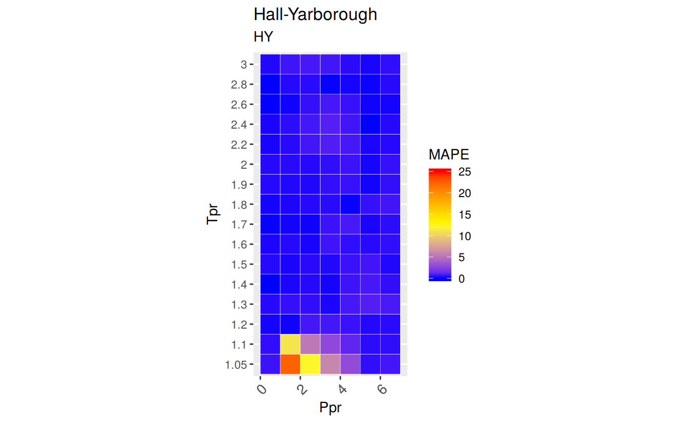
The Hall-Yarborough correlation shows a very high error at values of Tpr lower or equal than 1.1, being Tpr=1.05 the worst curve to calculate z values from. Keep that in mind. We will explore later a comparative tile chart where we confirm these early calculations.

Analyze the error for greater values of Tpr

Let’s see the numbers now for higher values of Tpr at various values of Ppr.

library(zFactor)
# enter vectors for Tpr and Ppr
tpr2 <- c(1.2, 1.3, 1.5, 2.0, 3.0) 
ppr2 <- c(0.5, 1.5, 2.5, 3.5, 4.5, 5.5) 
# get z values from the SK chart
z.chart <- getStandingKatzMatrix(ppr_vector = ppr2, tpr_vector = tpr2, pprRange = "lp")

# We do the same with the HY correlation:
# calculate z values at lower values of Tpr
z.calc <- z.HallYarborough(pres.pr = ppr2, temp.pr = tpr2) 
ape <- abs((z.calc - z.chart) / z.chart) * 100

# calculate the APE
cat("z.correlation \n"); print(z.calc)
cat("\n z.chart \n"); print(z.chart)
cat("\n APE \n"); print(ape)

z.correlation 
          0.5       1.5       2.5       3.5       4.5       5.5
1.2 0.8924176 0.6573432 0.5219634 0.5618489 0.6474310 0.7422294
1.3 0.9176300 0.7534433 0.6399020 0.6323003 0.6881127 0.7651710
1.5 0.9496855 0.8581232 0.7924067 0.7687902 0.7868071 0.8316848
2   0.9838234 0.9580002 0.9426939 0.9396286 0.9490995 0.9697839
3   1.0004261 1.0041806 1.0118999 1.0234786 1.0386327 1.0569640

 z.chart 
       0.5   1.5   2.5   3.5   4.5   5.5
1.20 0.893 0.657 0.519 0.565 0.650 0.741
1.30 0.916 0.756 0.638 0.633 0.684 0.759
1.50 0.948 0.859 0.794 0.770 0.790 0.836
2.00 0.982 0.956 0.941 0.937 0.945 0.969
3.00 1.002 1.009 1.018 1.029 1.041 1.056

 APE 
           0.5        1.5       2.5       3.5       4.5        5.5
1.2 0.06522262 0.05224243 0.5709802 0.5577242 0.3952245 0.16590798
1.3 0.17795221 0.33818375 0.2981152 0.1105437 0.6012676 0.81305005
1.5 0.17779256 0.10207082 0.2006642 0.1571161 0.4041660 0.51617648
2   0.18568379 0.20922900 0.1800061 0.2805309 0.4338140 0.08089785
3   0.15708015 0.47764307 0.5992268 0.5365750 0.2274063 0.09128453

At Tpr above or equal to 1.2 the HY correlation behaves very well.

Analyze the error at the isotherms

Now, let’s apply the function summary over the transpose of the matrix to observe the error of the correlation at each isotherm.

sum_t_ape <- summary(t(ape))
sum_t_ape

      1.2               1.3              1.5               2         
 Min.   :0.05224   Min.   :0.1105   Min.   :0.1021   Min.   :0.0809  
 1st Qu.:0.09039   1st Qu.:0.2080   1st Qu.:0.1623   1st Qu.:0.1814  
 Median :0.28057   Median :0.3181   Median :0.1892   Median :0.1975  
 Mean   :0.30122   Mean   :0.3899   Mean   :0.2597   Mean   :0.2284  
 3rd Qu.:0.51710   3rd Qu.:0.5355   3rd Qu.:0.3533   3rd Qu.:0.2627  
 Max.   :0.57098   Max.   :0.8131   Max.   :0.5162   Max.   :0.4338  
       3          
 Min.   :0.09128  
 1st Qu.:0.17466  
 Median :0.35252  
 Mean   :0.34820  
 3rd Qu.:0.52184  
 Max.   :0.59923  

In all, the error of z at these isotherms is less than 0.82%. Pretty good.

Prepare to plot SK chart values vs HY correlation

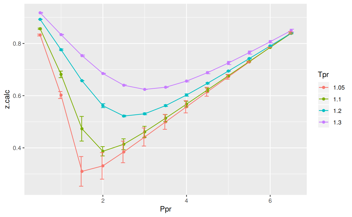
Now, we will be plotting the difference between the z values in the Standing-Katz and the z values calculated by Hall-Yarborough. For the moment let’s not pay attention to the numerical error but to the error bars in the plot (the orange bars).

library(zFactor)
library(tibble)
library(ggplot2)

tpr2 <- c(1.05, 1.1, 1.2, 1.3)
ppr2 <- c(0.5, 1.0, 1.5, 2, 2.5, 3.0, 3.5, 4.0, 4.5, 5.0, 5.5, 6.0, 6.5)

sk_corr_2 <- createTidyFromMatrix(ppr2, tpr2, correlation = "HY")
as_tibble(sk_corr_2)

p <- ggplot(sk_corr_2, aes(x=Ppr, y=z.calc, group=Tpr, color=Tpr)) +
    geom_line() +
    geom_point() +
    geom_errorbar(aes(ymin=z.calc-abs(dif), ymax=z.calc+abs(dif)), width=.4,
                  position=position_dodge(0.05))
print(p)

# A tibble: 52 x 5
   Tpr     Ppr z.chart z.calc       dif
   <chr> <dbl>   <dbl>  <dbl>     <dbl>
 1 1.05    0.5   0.829  0.832 -0.00347 
 2 1.1     0.5   0.854  0.857 -0.00250 
 3 1.2     0.5   0.893  0.892  0.000582
 4 1.3     0.5   0.916  0.918 -0.00163 
 5 1.05    1     0.589  0.602 -0.0134  
 6 1.1     1     0.669  0.682 -0.0126  
 7 1.2     1     0.779  0.776  0.00289 
 8 1.3     1     0.835  0.834  0.00104 
 9 1.05    1.5   0.253  0.310 -0.0569  
10 1.1     1.5   0.426  0.473 -0.0472  
# … with 42 more rows

As we were expecting, the errors can be found on Tpr=1.05 and Tpr=1.1

Analyzing the error for all the Tpr curves

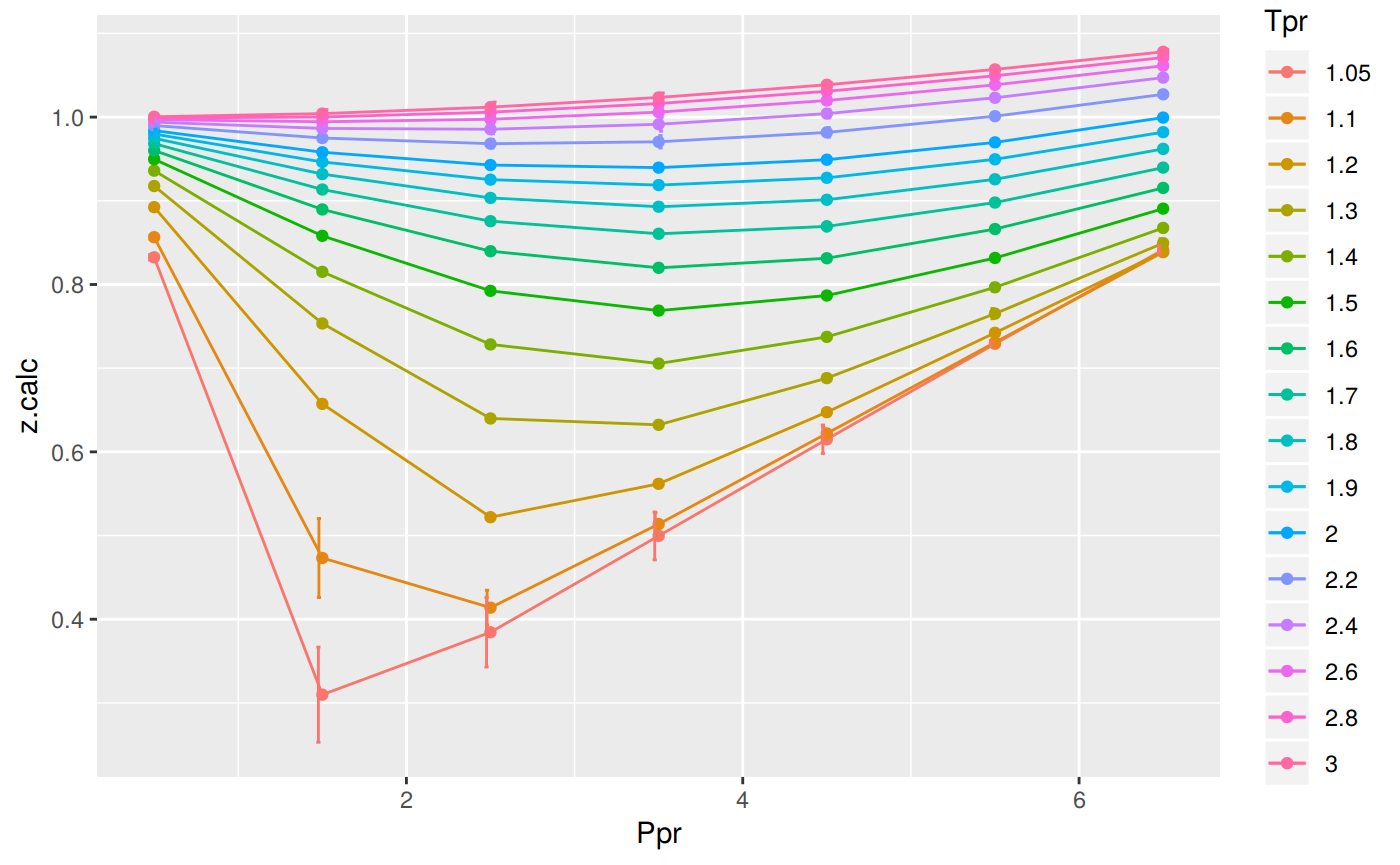
In this last example, we compare the values of z at all the isotherms. We use the function getCurvesDigitized in the zfactor package to obtain all the isotherms or Tpr curves in the Standing-Katz chart that have been digitized. The next function createTidyFromMatrix calculates z using the correlation and prepares a tidy dataset ready to plot.

library(ggplot2)
library(tibble)

# get all `lp` Tpr curves
tpr_all <- getStandingKatzTpr(pprRange = "lp")
ppr <- c(0.5, 1.5, 2.5, 3.5, 4.5, 5.5, 6.5) 
sk_corr_all <- createTidyFromMatrix(ppr, tpr_all, correlation = "HY")
as_tibble(sk_corr_all)

p <- ggplot(sk_corr_all, aes(x=Ppr, y=z.calc, group=Tpr, color=Tpr)) +
    geom_line() +
    geom_point() +
    geom_errorbar(aes(ymin=z.calc-dif, ymax=z.calc+dif), width=.4,
                  position=position_dodge(0.05))
print(p)

# A tibble: 112 x 5
   Tpr     Ppr z.chart z.calc        dif
   <chr> <dbl>   <dbl>  <dbl>      <dbl>
 1 1.05    0.5   0.829  0.832 -0.00347  
 2 1.1     0.5   0.854  0.857 -0.00250  
 3 1.2     0.5   0.893  0.892  0.000582 
 4 1.3     0.5   0.916  0.918 -0.00163  
 5 1.4     0.5   0.936  0.936  0.0000227
 6 1.5     0.5   0.948  0.950 -0.00169  
 7 1.6     0.5   0.959  0.960 -0.00114  
 8 1.7     0.5   0.968  0.968 -0.000255 
 9 1.8     0.5   0.974  0.975 -0.000640 
10 1.9     0.5   0.978  0.980 -0.00173  
# … with 102 more rows

As we saw before, we confirm that the greatest errors are localized in two of the Tpr curves: at 1.05 and 1.1.

Range of applicability of the correlation

What we will see here is the distribution of the Mean Average Percentage Error or MAPE accross all the Tpr isotherms and Ppr grids. Remember from the README: red and yellow are bad.

# MSE: Mean Squared Error
# RMSE: Root Mean Sqyared Error
# RSS: residual sum of square
# RMSLE: Root Mean Squared Logarithmic Error. Penalizes understimation.
# MAPE: Mean Absolute Percentage Error = AARE
# MPE: Mean Percentage error = ARE
# MAE: Mean Absolute Error
library(dplyr)
grouped <- group_by(sk_corr_all, Tpr, Ppr)
smry_tpr_ppr <- summarise(grouped, 
          RMSE= sqrt(mean((z.chart-z.calc)^2)), 
          MPE = sum((z.calc - z.chart) / z.chart) * 100 / n(),
          MAPE = sum(abs((z.calc - z.chart) / z.chart)) * 100 / n(), 
          MSE = sum((z.calc - z.chart)^2) / n(), 
          RSS = sum((z.calc - z.chart)^2),
          MAE = sum(abs(z.calc - z.chart)) / n(),
          RMLSE = sqrt(1/n()*sum((log(z.calc +1)-log(z.chart +1))^2))
          )

ggplot(smry_tpr_ppr, aes(Ppr, Tpr)) + 
    geom_tile(data=smry_tpr_ppr, aes(fill=MAPE), color="white") +
    scale_fill_gradient2(low="blue", high="red", mid="yellow", na.value = "pink",
                         midpoint=12.5, limit=c(0, 25), name="MAPE") + 
    theme(axis.text.x = element_text(angle=45, vjust=1, size=11, hjust=1)) + 
    coord_equal() +
    ggtitle("Hall-Yarborough", subtitle = "HY")

Plotting the Tpr and Ppr values that show more error

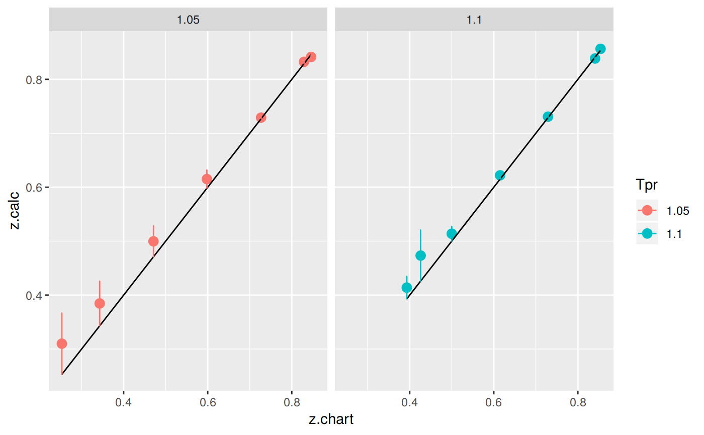
This is just plotting the couple of isotherms where we see the largest errors.

library(dplyr)

sk_corr_all %>%
    filter(Tpr %in% c("1.05", "1.1")) %>%
    ggplot(aes(x = z.chart, y=z.calc, group = Tpr, color = Tpr)) +
    geom_point(size = 3) +
    geom_line(aes(x = z.chart, y = z.chart), color = "black") +
    facet_grid(. ~ Tpr) +
    geom_errorbar(aes(ymin=z.calc-abs(dif), ymax=z.calc+abs(dif)),
                  position=position_dodge(0.05))

Looking numerically at the errors

Finally, the dataframe with the calculated errors between the z from the correlation and the z read from the chart:

as_tibble(smry_tpr_ppr)

# A tibble: 112 x 9
   Tpr     Ppr    RMSE    MPE   MAPE        MSE        RSS     MAE   RMLSE
   <chr> <dbl>   <dbl>  <dbl>  <dbl>      <dbl>      <dbl>   <dbl>   <dbl>
 1 1.05    0.5 0.00347  0.418  0.418 0.0000120  0.0000120  0.00347 0.00189
 2 1.05    1.5 0.0569  22.5   22.5   0.00324    0.00324    0.0569  0.0444 
 3 1.05    2.5 0.0415  12.1   12.1   0.00172    0.00172    0.0415  0.0304 
 4 1.05    3.5 0.0286   6.08   6.08  0.000819   0.000819   0.0286  0.0193 
 5 1.05    4.5 0.0171   2.86   2.86  0.000292   0.000292   0.0171  0.0106 
 6 1.05    5.5 0.00210  0.289  0.289 0.00000442 0.00000442 0.00210 0.00122
 7 1.05    6.5 0.00447 -0.528  0.528 0.0000200  0.0000200  0.00447 0.00242
 8 1.1     0.5 0.00250  0.293  0.293 0.00000627 0.00000627 0.00250 0.00135
 9 1.1     1.5 0.0472  11.1   11.1   0.00223    0.00223    0.0472  0.0326 
10 1.1     2.5 0.0209   5.31   5.31  0.000435   0.000435   0.0209  0.0149 
# … with 102 more rows

RMSE: Root Mean Square Error

\[RMSE = \sqrt {\frac {1}{n} \sum_{i=1}^{n} (y_i - \hat y_i)^2}\]

Appendix

getStandingKatzMatrix is equivalent to using the sapply function with the internal function .z.HallYarborough (the dot means it’s internal), which we call adding the prefix zFactor:::. That is, the package name and three colons.

# test HY with 1st-derivative using the values from the paper 
 
ppr <- c(0.5, 1.5, 2.5, 3.5, 4.5, 5.5, 6.5) 
tpr <- c(1.3, 1.5, 1.7, 2) 
 
hy <- sapply(ppr, function(x)  
    sapply(tpr, function(y) zFactor:::.z.HallYarborough(pres.pr = x, temp.pr = y))) 
 
rownames(hy) <- tpr 
colnames(hy) <- ppr 
print(hy) 

          0.5       1.5       2.5       3.5       4.5       5.5       6.5
1.3 0.9176300 0.7534433 0.6399020 0.6323003 0.6881127 0.7651710 0.8493794
1.5 0.9496855 0.8581232 0.7924067 0.7687902 0.7868071 0.8316848 0.8906351
1.7 0.9682547 0.9134862 0.8756412 0.8605668 0.8694525 0.8978885 0.9396353
2   0.9838234 0.9580002 0.9426939 0.9396286 0.9490995 0.9697839 0.9994317

References

Hall, Kenneth R, and Lyman Yarborough. 1973. “A New Equation of State for Z-Factor Calculations.” Oil and Gas Journal 71 (7): 82–92.