16 sklearn
This is a machine learning library.
16.2 The Library
sklearn does not automatically import its subpackages. Therefore all subpakcages must be specifically loaded before use.
# Sample Data
from sklearn                 import datasets

# Model Selection
from sklearn.model_selection import train_test_split
from sklearn.model_selection import KFold
from sklearn.model_selection import LeaveOneOut
from sklearn.model_selection import cross_validate

# Preprocessing
# from sklearn.preprocessing   import Imputer
from sklearn.impute import SimpleImputer

from sklearn.preprocessing   import MinMaxScaler
from sklearn.preprocessing   import StandardScaler
from sklearn.preprocessing   import Normalizer
from sklearn.preprocessing   import PolynomialFeatures

# Model and Pipeline
from sklearn.linear_model    import LinearRegression,Lasso
from sklearn.pipeline        import make_pipeline

# Measurement
from sklearn.metrics         import *

import statsmodels.formula.api as smf
16.3 Model Fitting
split
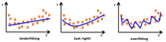
16.3.1 Underfitting
- The model does not fit the training data and therefore misses the trends in the data
- The model cannot be generalized to new data, this is usually the result of a very simple model (not enough predictors/independent variables)
- The model will have poor predictive ability
- For example, we fit a linear model (like linear regression) to data that is not linear
16.3.2 Overfitting
- The model has trained ?too well? and is now, well, fit too closely to the training dataset
- The model is too complex (i.e. too many features/variables compared to the number of observations)
- The model will be very accurate on the training data but will probably be very not accurate on untrained or new data
- The model is not generalized (or not AS generalized), meaning you can generalize the results
- The model learns or describes the ?noise? in the training data instead of the actual relationships between variables in the data
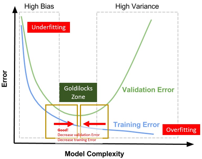
16.4 Model Tuning
- A highly complex model tend to overfit
- A too flexible model tend to underfit
Complexity can be reduced by: - Less features - Less degree of polynomial features - Apply generalization (tuning hyperparameters)
split
16.6 Built-in Datasets
sklearn included some popular datasets to play with
Each dataset is of type Bunch.
It has useful data (array) in the form of properties:
- keys (display all data availabe within the dataset)
- data (common)
- target (common)
- DESCR (common)
- feature_names (some dataset)
- target_names (some dataset)
- images (some dataset)
16.6.1 diabetes (regression)
16.6.1.1 Load Dataset
diabetes = datasets.load_diabetes()
print (type(diabetes))
#:> <class 'sklearn.utils.Bunch'>16.6.1.2 keys
diabetes.keys()#:> dict_keys(['data', 'target', 'frame', 'DESCR', 'feature_names', 'data_filename', 'target_filename'])16.6.1.3 Features and Target
.data = features - two dimension array
.target = target - one dimension array
print (type(diabetes.data))#:> <class 'numpy.ndarray'>print (type(diabetes.target))#:> <class 'numpy.ndarray'>print (diabetes.data.shape)#:> (442, 10)print (diabetes.target.shape)#:> (442,)16.6.2 digits (Classification)
This is a copy of the test set of the UCI ML hand-written digits datasets
digits = datasets.load_digits()
print (type(digits))
#:> <class 'sklearn.utils.Bunch'>print (type(digits.data))#:> <class 'numpy.ndarray'>digits.keys()#:> dict_keys(['data', 'target', 'frame', 'feature_names', 'target_names', 'images', 'DESCR'])digits.target_names#:> array([0, 1, 2, 3, 4, 5, 6, 7, 8, 9])16.6.2.2 Images
- images is 3 dimensional array
- There are 1797 samples, each sample is 8x8 pixels
digits.images.shape#:> (1797, 8, 8)type(digits.images)#:> <class 'numpy.ndarray'>Each element represent the data that make its target
print (digits.target[100])#:> 4print (digits.images[100])#:> [[ 0. 0. 0. 2. 13. 0. 0. 0.]
#:> [ 0. 0. 0. 8. 15. 0. 0. 0.]
#:> [ 0. 0. 5. 16. 5. 2. 0. 0.]
#:> [ 0. 0. 15. 12. 1. 16. 4. 0.]
#:> [ 0. 4. 16. 2. 9. 16. 8. 0.]
#:> [ 0. 0. 10. 14. 16. 16. 4. 0.]
#:> [ 0. 0. 0. 0. 13. 8. 0. 0.]
#:> [ 0. 0. 0. 0. 13. 6. 0. 0.]]plt.matshow(digits.images[100]) 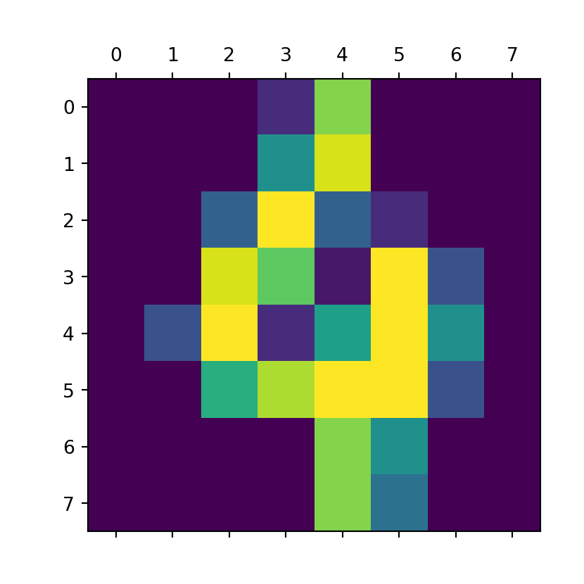
16.6.3 iris (Classification)
iris = datasets.load_iris()iris.keys()#:> dict_keys(['data', 'target', 'frame', 'target_names', 'DESCR', 'feature_names', 'filename'])16.6.3.1 Feature Names
iris.feature_names#:> ['sepal length (cm)', 'sepal width (cm)', 'petal length (cm)', 'petal width (cm)']16.6.3.2 target
iris.target_names#:> array(['setosa', 'versicolor', 'virginica'], dtype='<U10')iris.target#:> array([0, 0, 0, 0, 0, 0, 0, 0, 0, 0, 0, 0, 0, 0, 0, 0, 0, 0, 0, 0, 0, 0,
#:> 0, 0, 0, 0, 0, 0, 0, 0, 0, 0, 0, 0, 0, 0, 0, 0, 0, 0, 0, 0, 0, 0,
#:> 0, 0, 0, 0, 0, 0, 1, 1, 1, 1, 1, 1, 1, 1, 1, 1, 1, 1, 1, 1, 1, 1,
#:> 1, 1, 1, 1, 1, 1, 1, 1, 1, 1, 1, 1, 1, 1, 1, 1, 1, 1, 1, 1, 1, 1,
#:> 1, 1, 1, 1, 1, 1, 1, 1, 1, 1, 1, 1, 2, 2, 2, 2, 2, 2, 2, 2, 2, 2,
#:> 2, 2, 2, 2, 2, 2, 2, 2, 2, 2, 2, 2, 2, 2, 2, 2, 2, 2, 2, 2, 2, 2,
#:> 2, 2, 2, 2, 2, 2, 2, 2, 2, 2, 2, 2, 2, 2, 2, 2, 2, 2])16.7 Train Test Data Splitting
16.7.1 Sample Data
Generate 100 rows of data, with 3x features (X1,X2,X3), and one dependant variable (Y)
n = 21  # number of samples
I = 5  # intercept value
E = np.random.randint( 1,20, n)  # Error
x1 = np.random.randint( 1,n+1, n)
x2 = np.random.randint( 1,n+1, n)
x3 = np.random.randint( 1,n+1, n)
y = 0.1*x1 + 0.2*x2 + 0.3*x3 + E + I
mydf = pd.DataFrame({
    'y':y,
    'x1':x1,
    'x2':x2,
    'x3':x3
})
mydf.shape
#:> (21, 4)16.7.2 One Time Split
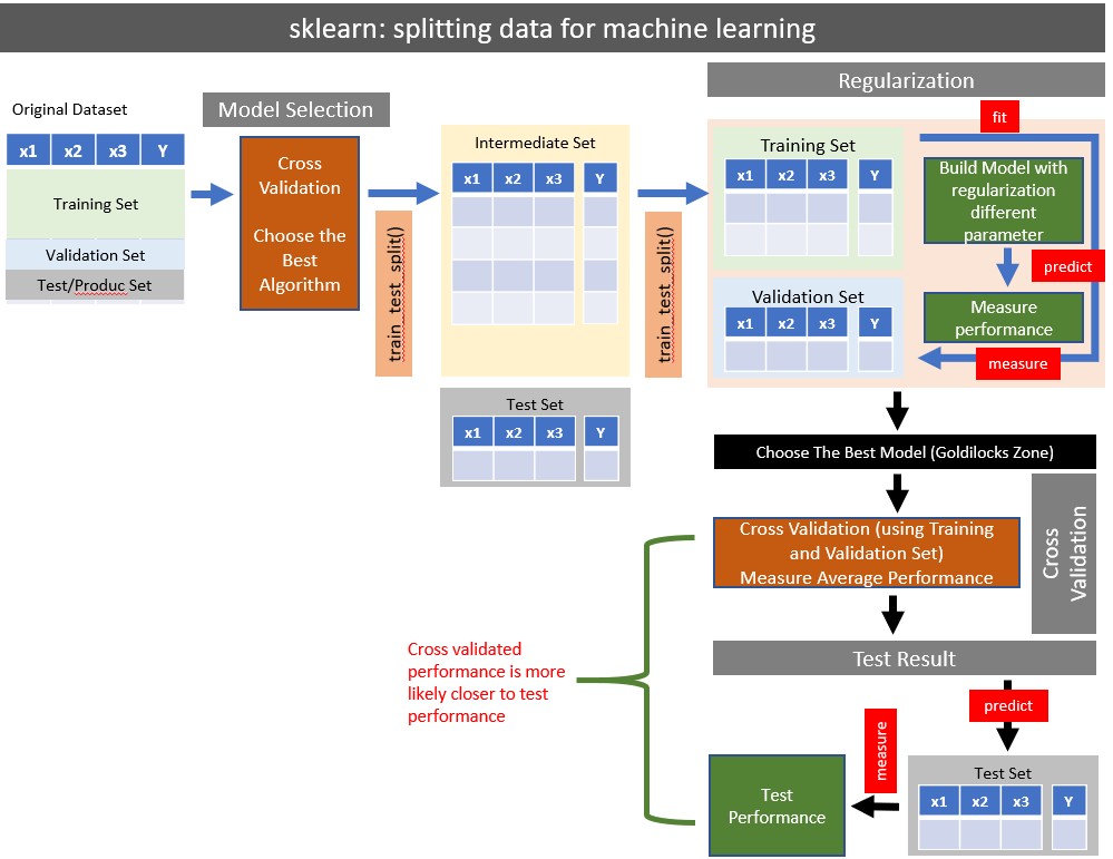
sklearn::train_test_split() has two forms: - Take one DF, split into 2 DF (most of sklearn modeling use this method - Take two DFs, split into 4 DF
mydf.head()#:> y x1 x2 x3
#:> 0 34.9 17 21 20
#:> 1 13.0 5 3 3
#:> 2 26.4 13 17 9
#:> 3 26.4 21 9 15
#:> 4 17.9 17 4 1816.7.2.1 Method 1: Split One Dataframe Into Two (Train & Test)
traindf, testdf = train_test_split( df, test_size=, random_state= )
 # random_state : seed number (integer), optional
 # test_size    : fraction of 1, 0.2 means 20%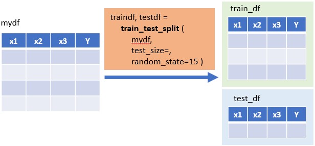
split
traindf, testdf = train_test_split(mydf,test_size=0.2, random_state=25)print (len(traindf))#:> 16print (len(testdf))#:> 516.7.2.2 Method 2: Split Two DataFrame (X,Y) into Four x_train/test, y_train/test
x_train, x_test, y_train, y_test = train_test_split( X,Y, test_size=, random_state= )
 # random_state : seed number (integer), optional
 # test_size    : fraction of 1, 0.2 means 20%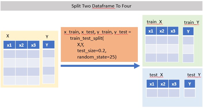
split
Split DataFrame into X and Y First
feature_cols = ['x1','x2','x3']
X = mydf[feature_cols]
Y = mydf.y
Then Split X/Y into x_train/test, y_train/test
x_train, x_test, y_train, y_test = train_test_split( X,Y, test_size=0.2, random_state=25)
print (len(x_train))
#:> 16print (len(x_test))#:> 516.7.3 K-Fold
KFold(n_splits=3, shuffle=False, random_state=None)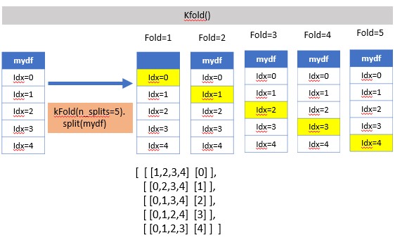
split
suffle=False (default), meaning index number is taken continously
kf = KFold(n_splits=7)for train_index, test_index in kf.split(X):
print (train_index, test_index)#:> [ 3 4 5 6 7 8 9 10 11 12 13 14 15 16 17 18 19 20] [0 1 2]
#:> [ 0 1 2 6 7 8 9 10 11 12 13 14 15 16 17 18 19 20] [3 4 5]
#:> [ 0 1 2 3 4 5 9 10 11 12 13 14 15 16 17 18 19 20] [6 7 8]
#:> [ 0 1 2 3 4 5 6 7 8 12 13 14 15 16 17 18 19 20] [ 9 10 11]
#:> [ 0 1 2 3 4 5 6 7 8 9 10 11 15 16 17 18 19 20] [12 13 14]
#:> [ 0 1 2 3 4 5 6 7 8 9 10 11 12 13 14 18 19 20] [15 16 17]
#:> [ 0 1 2 3 4 5 6 7 8 9 10 11 12 13 14 15 16 17] [18 19 20]shuffle=True
kf = KFold(n_splits=7, shuffle=True)for train_index, test_index in kf.split(X):
print (train_index, test_index)#:> [ 0 1 2 3 4 5 7 8 9 10 11 12 13 14 16 17 19 20] [ 6 15 18]
#:> [ 0 1 3 4 5 6 7 8 9 10 12 13 14 15 16 17 18 19] [ 2 11 20]
#:> [ 0 1 2 5 6 7 8 9 10 11 12 13 14 15 17 18 19 20] [ 3 4 16]
#:> [ 0 1 2 3 4 5 6 7 9 10 11 14 15 16 17 18 19 20] [ 8 12 13]
#:> [ 1 2 3 4 5 6 7 8 9 10 11 12 13 14 15 16 18 20] [ 0 17 19]
#:> [ 0 2 3 4 6 7 8 9 11 12 13 14 15 16 17 18 19 20] [ 1 5 10]
#:> [ 0 1 2 3 4 5 6 8 10 11 12 13 15 16 17 18 19 20] [ 7 9 14]16.7.4 Leave One Out
- For a dataset of N rows, Leave One Out will split N-1 times, each time leaving one row as test, remaning as training set.
- Due to the high number of test sets (which is the same as the number of samples-1) this cross-validation method can be very costly. For large datasets one should favor KFold.
loo = LeaveOneOut()for train_index, test_index in loo.split(X):
print (train_index, test_index)#:> [ 1 2 3 4 5 6 7 8 9 10 11 12 13 14 15 16 17 18 19 20] [0]
#:> [ 0 2 3 4 5 6 7 8 9 10 11 12 13 14 15 16 17 18 19 20] [1]
#:> [ 0 1 3 4 5 6 7 8 9 10 11 12 13 14 15 16 17 18 19 20] [2]
#:> [ 0 1 2 4 5 6 7 8 9 10 11 12 13 14 15 16 17 18 19 20] [3]
#:> [ 0 1 2 3 5 6 7 8 9 10 11 12 13 14 15 16 17 18 19 20] [4]
#:> [ 0 1 2 3 4 6 7 8 9 10 11 12 13 14 15 16 17 18 19 20] [5]
#:> [ 0 1 2 3 4 5 7 8 9 10 11 12 13 14 15 16 17 18 19 20] [6]
#:> [ 0 1 2 3 4 5 6 8 9 10 11 12 13 14 15 16 17 18 19 20] [7]
#:> [ 0 1 2 3 4 5 6 7 9 10 11 12 13 14 15 16 17 18 19 20] [8]
#:> [ 0 1 2 3 4 5 6 7 8 10 11 12 13 14 15 16 17 18 19 20] [9]
#:> [ 0 1 2 3 4 5 6 7 8 9 11 12 13 14 15 16 17 18 19 20] [10]
#:> [ 0 1 2 3 4 5 6 7 8 9 10 12 13 14 15 16 17 18 19 20] [11]
#:> [ 0 1 2 3 4 5 6 7 8 9 10 11 13 14 15 16 17 18 19 20] [12]
#:> [ 0 1 2 3 4 5 6 7 8 9 10 11 12 14 15 16 17 18 19 20] [13]
#:> [ 0 1 2 3 4 5 6 7 8 9 10 11 12 13 15 16 17 18 19 20] [14]
#:> [ 0 1 2 3 4 5 6 7 8 9 10 11 12 13 14 16 17 18 19 20] [15]
#:> [ 0 1 2 3 4 5 6 7 8 9 10 11 12 13 14 15 17 18 19 20] [16]
#:> [ 0 1 2 3 4 5 6 7 8 9 10 11 12 13 14 15 16 18 19 20] [17]
#:> [ 0 1 2 3 4 5 6 7 8 9 10 11 12 13 14 15 16 17 19 20] [18]
#:> [ 0 1 2 3 4 5 6 7 8 9 10 11 12 13 14 15 16 17 18 20] [19]
#:> [ 0 1 2 3 4 5 6 7 8 9 10 11 12 13 14 15 16 17 18 19] [20]X#:> x1 x2 x3
#:> 0 17 21 20
#:> 1 5 3 3
#:> 2 13 17 9
#:> 3 21 9 15
#:> 4 17 4 18
#:> .. .. .. ..
#:> 16 15 3 10
#:> 17 15 20 12
#:> 18 17 6 11
#:> 19 14 13 16
#:> 20 8 1 10
#:>
#:> [21 rows x 3 columns]16.8 Polynomial Transform
This can be used as part of feature engineering, to introduce new features for data that seems to fit with quadradic model.
16.8.1 Single Variable
16.8.1.1 Sample Data
Data must be 2-D before polynomial features can be applied. Code below convert 1D array into 2D array.
x = np.array([1, 2, 3, 4, 5])
X = x[:,np.newaxis]
X
#:> array([[1],
#:> [2],
#:> [3],
#:> [4],
#:> [5]])16.8.1.2 Degree 1
One Degree means maintain original features. No new features is created.
PolynomialFeatures(degree=1, include_bias=False).fit_transform(X)#:> array([[1.],
#:> [2.],
#:> [3.],
#:> [4.],
#:> [5.]])16.8.1.3 Degree 2
Degree-1 original feature: x
Degree-2 additional features: x^2
PolynomialFeatures(degree=2, include_bias=False).fit_transform(X)#:> array([[ 1., 1.],
#:> [ 2., 4.],
#:> [ 3., 9.],
#:> [ 4., 16.],
#:> [ 5., 25.]])16.8.1.4 Degree 3
Degree-1 original feature: x
Degree-2 additional features: x^2
Degree-3 additional features: x^3
PolynomialFeatures(degree=3, include_bias=False).fit_transform(X)#:> array([[ 1., 1., 1.],
#:> [ 2., 4., 8.],
#:> [ 3., 9., 27.],
#:> [ 4., 16., 64.],
#:> [ 5., 25., 125.]])16.8.1.5 Degree 4
Degree-1 original feature: x
Degree-2 additional features: x^2
Degree-3 additional features: x^3
Degree-3 additional features: x^4
PolynomialFeatures(degree=4, include_bias=False).fit_transform(X)#:> array([[ 1., 1., 1., 1.],
#:> [ 2., 4., 8., 16.],
#:> [ 3., 9., 27., 81.],
#:> [ 4., 16., 64., 256.],
#:> [ 5., 25., 125., 625.]])16.8.2 Two Variables
16.8.2.1 Sample Data
X = pd.DataFrame( {'x1': [1, 2, 3, 4, 5 ],
                   'x2': [6, 7, 8, 9, 10]})
X
#:> x1 x2
#:> 0 1 6
#:> 1 2 7
#:> 2 3 8
#:> 3 4 9
#:> 4 5 1016.8.2.2 Degree 2
Degree-1 original   features:  x1,     x2
Degree-2 additional features: x1^2, x2^2, x1:x2 PolynomialFeatures(degree=2, include_bias=False).fit_transform(X)#:> array([[ 1., 6., 1., 6., 36.],
#:> [ 2., 7., 4., 14., 49.],
#:> [ 3., 8., 9., 24., 64.],
#:> [ 4., 9., 16., 36., 81.],
#:> [ 5., 10., 25., 50., 100.]])16.8.2.3 Degree 3
Degree-1 original   features:  x1,       x2
Degree-2 additional features:  x1^2,     x2^2,   x1:x2
Degree-3 additional features: x1^3, x2^3 x1:x2^2 x2:x1^2PolynomialFeatures(degree=3, include_bias=False).fit_transform(X)#:> array([[ 1., 6., 1., 6., 36., 1., 6., 36., 216.],
#:> [ 2., 7., 4., 14., 49., 8., 28., 98., 343.],
#:> [ 3., 8., 9., 24., 64., 27., 72., 192., 512.],
#:> [ 4., 9., 16., 36., 81., 64., 144., 324., 729.],
#:> [ 5., 10., 25., 50., 100., 125., 250., 500., 1000.]])16.9 Imputation of Missing Data
16.10 Scaling
It is possible that some insignificant variable with larger range will be dominating the objective function.
We can remove this problem by scaling down all the features to a same range.
16.10.1 Sample Data
X=mydf.filter(like='x')[:5]
X
#:> x1 x2 x3
#:> 0 17 21 20
#:> 1 5 3 3
#:> 2 13 17 9
#:> 3 21 9 15
#:> 4 17 4 1816.10.2 MinMax Scaler
MinMaxScaler( feature_range(0,1), copy=True )
# default feature range (output result) from 0 to 1
# default return a copy of new array, copy=False will inplace original array
Define Scaler Object
scaler = MinMaxScaler()Transform Data
scaler.fit_transform(X)#:> array([[0.75 , 1. , 1. ],
#:> [0. , 0. , 0. ],
#:> [0.5 , 0.77777778, 0.35294118],
#:> [1. , 0.33333333, 0.70588235],
#:> [0.75 , 0.05555556, 0.88235294]])Scaler Attributes
data_min_: minimum value of the feature (before scaling)
data_max_: maximum value of the feature (before scaling) pd.DataFrame(list(zip(scaler.data_min_, scaler.data_max_)),
columns=['data_min','data_max'],
index=X.columns)#:> data_min data_max
#:> x1 5.0 21.0
#:> x2 3.0 21.0
#:> x3 3.0 20.016.10.3 Standard Scaler
It is most suitable for techniques that assume a Gaussian distribution in the input variables and work better with rescaled data, such as linear regression, logistic regression and linear discriminate analysis.
StandardScaler(copy=True, with_mean=True, with_std=True)
# copy=True : return a copy of data, instead of inplace
# with_mean=True : centre all features by substracting with its mean
# with_std=True  : centre all features by dividing with its std
Define Scaler Object
scaler = StandardScaler()Transform Data
scaler.fit_transform(X)#:> array([[ 0.44232587, 1.43448707, 1.12378227],
#:> [-1.76930347, -1.0969607 , -1.60540325],
#:> [-0.29488391, 0.87194312, -0.6421613 ],
#:> [ 1.17953565, -0.25314478, 0.32108065],
#:> [ 0.44232587, -0.95632472, 0.80270162]])Scaler Attributes
After the data transformation step above, scaler will have the mean and variance information for each feature.
pd.DataFrame(list(zip(scaler.mean_, scaler.var_)),
             columns=['mean','variance'],
             index=X.columns)
#:> mean variance
#:> x1 14.6 29.44
#:> x2 10.8 50.56
#:> x3 13.0 38.8016.11 Pipeline
With any of the preceding examples, it can quickly become tedious to do the transformations by hand, especially if you wish to string together multiple steps. For example, we might want a processing pipeline that looks something like this:
-
Impute missing values using the mean
-
Transform features to quadratic
- Fit a linear regression
make_pipeline takes list of functions as parameters. When calling fit() on a pipeline object, these functions will be performed in sequential with data flow from one function to another.
make_pipeline (
    function_1 (),
    function_2 (),
    function_3 ()
 )
16.11.1 Sample Data
X#:> x1 x2 x3
#:> 0 17 21 20
#:> 1 5 3 3
#:> 2 13 17 9
#:> 3 21 9 15
#:> 4 17 4 18y#:> array([14, 16, -1, 8, -5])16.11.2 Create Pipeline
my_pipe = make_pipeline (
    SimpleImputer            (strategy='mean'),
    PolynomialFeatures (degree=2),
    LinearRegression   ()
)
type(my_pipe)
#:> <class 'sklearn.pipeline.Pipeline'>my_pipe#:> Pipeline(steps=[('simpleimputer', SimpleImputer()),
#:> ('polynomialfeatures', PolynomialFeatures()),
#:> ('linearregression', LinearRegression())])16.11.3 Executing Pipeline
my_pipe.fit( X, y) # execute the pipeline#:> Pipeline(steps=[('simpleimputer', SimpleImputer()),
#:> ('polynomialfeatures', PolynomialFeatures()),
#:> ('linearregression', LinearRegression())])print (y)#:> [14 16 -1 8 -5]print (my_pipe.predict(X))#:> [14. 16. -1. 8. -5.]type(my_pipe)#:> <class 'sklearn.pipeline.Pipeline'>16.12 Cross Validation
16.12.3 Run Cross Validation
Single Scorer
Use default scorer of the estimator (if available)
lasso = Lasso()
cv_results1 = cross_validate(lasso, X,y,cv=kf,
    return_train_score=False)
Multiple Scorer
Specify the scorer
http://scikit-learn.org/stable/modules/model_evaluation.html#scoring-parameter
cv_results2 = cross_validate(lasso, X,y,cv=kf,
    scoring=("neg_mean_absolute_error","neg_mean_squared_error","r2"),
    return_train_score=False)
16.12.4 The Result
Result is a dictionary
cv_results1.keys()#:> dict_keys(['fit_time', 'score_time', 'test_score'])cv_results2.keys()#:> dict_keys(['fit_time', 'score_time', 'test_neg_mean_absolute_error', 'test_neg_mean_squared_error', 'test_r2'])cv_results1#:> {'fit_time': array([0.00107646, 0.00174236, 0.0007472 , 0.00078654, 0.00084043]), 'score_time': array([0.0008533 , 0.00060225, 0.00101304, 0.00054669, 0.00101948]), 'test_score': array([0.28349047, 0.35157959, 0.3533813 , 0.33481474, 0.36453281])}cv_results2#:> {'fit_time': array([0.00155902, 0.00112081, 0.00144434, 0.0011692 , 0.00112915]), 'score_time': array([0.00154161, 0.0016377 , 0.00273466, 0.00171494, 0.00147605]), 'test_neg_mean_absolute_error': array([-50.09003423, -52.54110842, -55.02813846, -50.81121806,
#:> -55.60471593]), 'test_neg_mean_squared_error': array([-3491.74009759, -4113.86002091, -4046.91780932, -3489.74018715,
#:> -4111.92401769]), 'test_r2': array([0.28349047, 0.35157959, 0.3533813 , 0.33481474, 0.36453281])}