14 matplotlib
14.1 Library
import matplotlib
import matplotlib.pyplot as plt
import seaborn as sns
import numpy as np

from plydata import define, query, select, group_by, summarize, arrange, head, rename
import plotnine
from plotnine import *
14.2 Sample Data
This chapter uses the sample data generate with below code. The idea is to simulate two categorical-alike feature, and two numeric value feature:
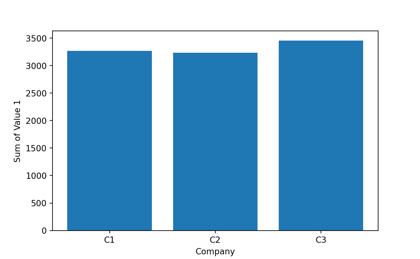
- com is random character between ?C1?, ?C2? and ?C3?
- dept is random character between ?D1?, ?D2?, ?D3?, ?D4? and ?D5?
- grp is random character with randomly generated ?G1?, ?G2?
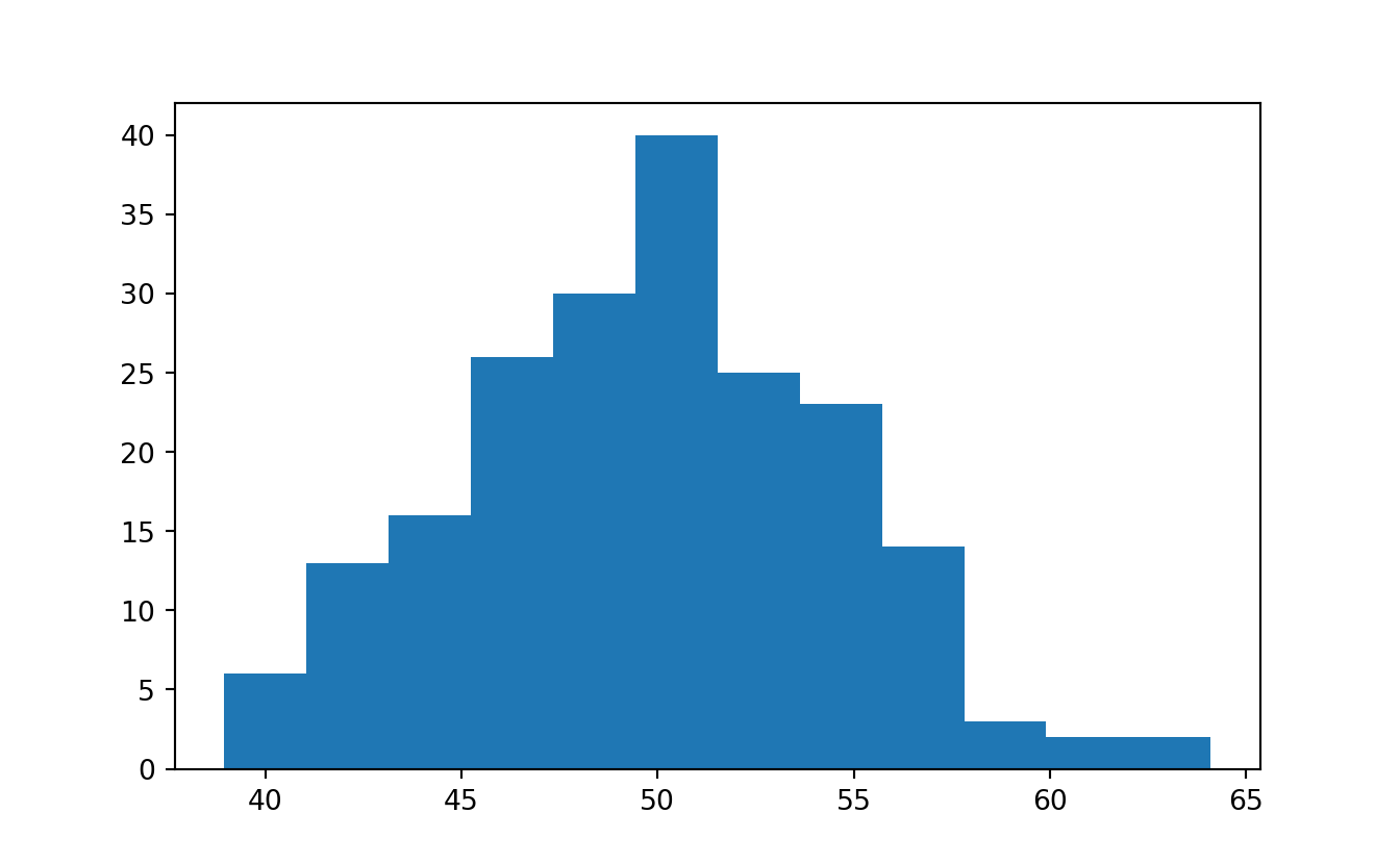
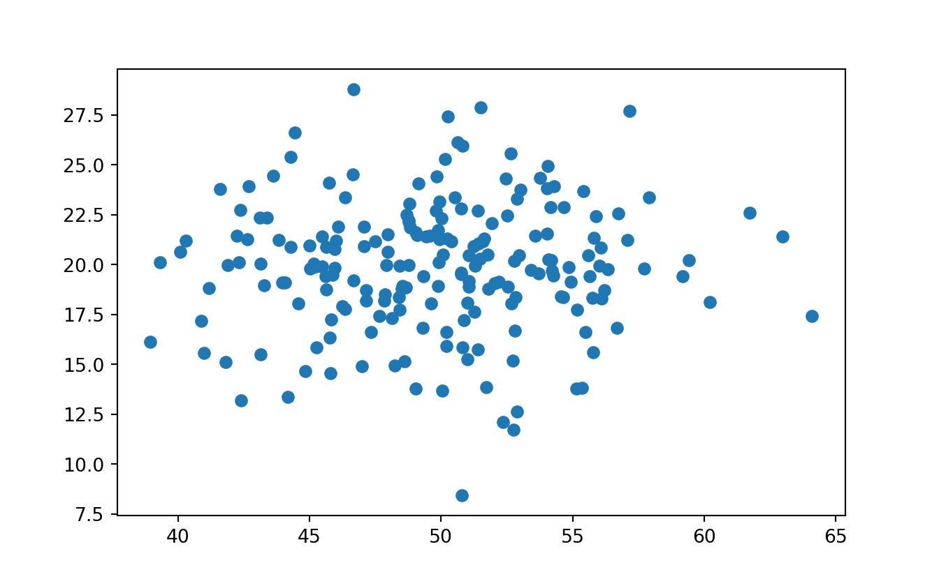
- value1 represents numeric value, normally distributed at mean 50
- value2 is numeric value, normally distributed at mean 25
n = 200
comp = ['C' + i for i in np.random.randint( 1,4, size  = n).astype(str)] # 3x Company
dept = ['D' + i for i in np.random.randint( 1,6, size  = n).astype(str)] # 5x Department
grp =  ['G' + i for i in np.random.randint( 1,3, size  = n).astype(str)] # 2x Groups
value1 = np.random.normal( loc=50 , scale=5 , size = n)
value2 = np.random.normal( loc=20 , scale=3 , size = n)
value3 = np.random.normal( loc=5 , scale=30 , size = n)

mydf = pd.DataFrame({
    'comp':comp,
    'dept':dept,
    'grp': grp,
    'value1':value1,
    'value2':value2,
    'value3':value3 })
mydf.head()
#:> comp dept grp value1 value2 value3
#:> 0 C1 D3 G1 47.343508 16.623546 1.741223
#:> 1 C2 D1 G1 61.737449 22.592145 29.889468
#:> 2 C2 D4 G1 48.773299 22.211320 17.476382
#:> 3 C2 D2 G1 47.856641 18.504218 35.166332
#:> 4 C3 D3 G1 51.066041 19.154196 -2.138135mydf.info()#:> <class 'pandas.core.frame.DataFrame'>
#:> RangeIndex: 200 entries, 0 to 199
#:> Data columns (total 6 columns):
#:> # Column Non-Null Count Dtype
#:> --- ------ -------------- -----
#:> 0 comp 200 non-null object
#:> 1 dept 200 non-null object
#:> 2 grp 200 non-null object
#:> 3 value1 200 non-null float64
#:> 4 value2 200 non-null float64
#:> 5 value3 200 non-null float64
#:> dtypes: float64(3), object(3)
#:> memory usage: 9.5+ KB14.3 MATLAB-like API
- The good thing about the pylab MATLAB-style API is that it is easy to get started with if you are familiar with MATLAB, and it has a minumum of coding overhead for simple plots.
- However, I’d encourrage not using the MATLAB compatible API for anything but the simplest figures.
- Instead, I recommend learning and using matplotlib’s object-oriented plotting API. It is remarkably powerful. For advanced figures with subplots, insets and other components it is very nice to work with.
14.4 Object-Oriented API
14.4.2 Single Plot
One figure, one axes
fig = plt.figure()
axes = fig.add_axes([0,0,1,1]) # left, bottom, width, height (range 0 to 1)
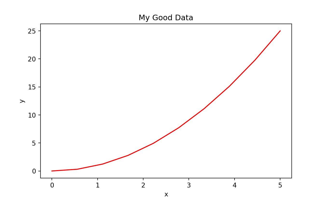
axes.plot(x, y, 'r')
axes.set_xlabel('x')
axes.set_ylabel('y')
axes.set_title('title')
plt.show()
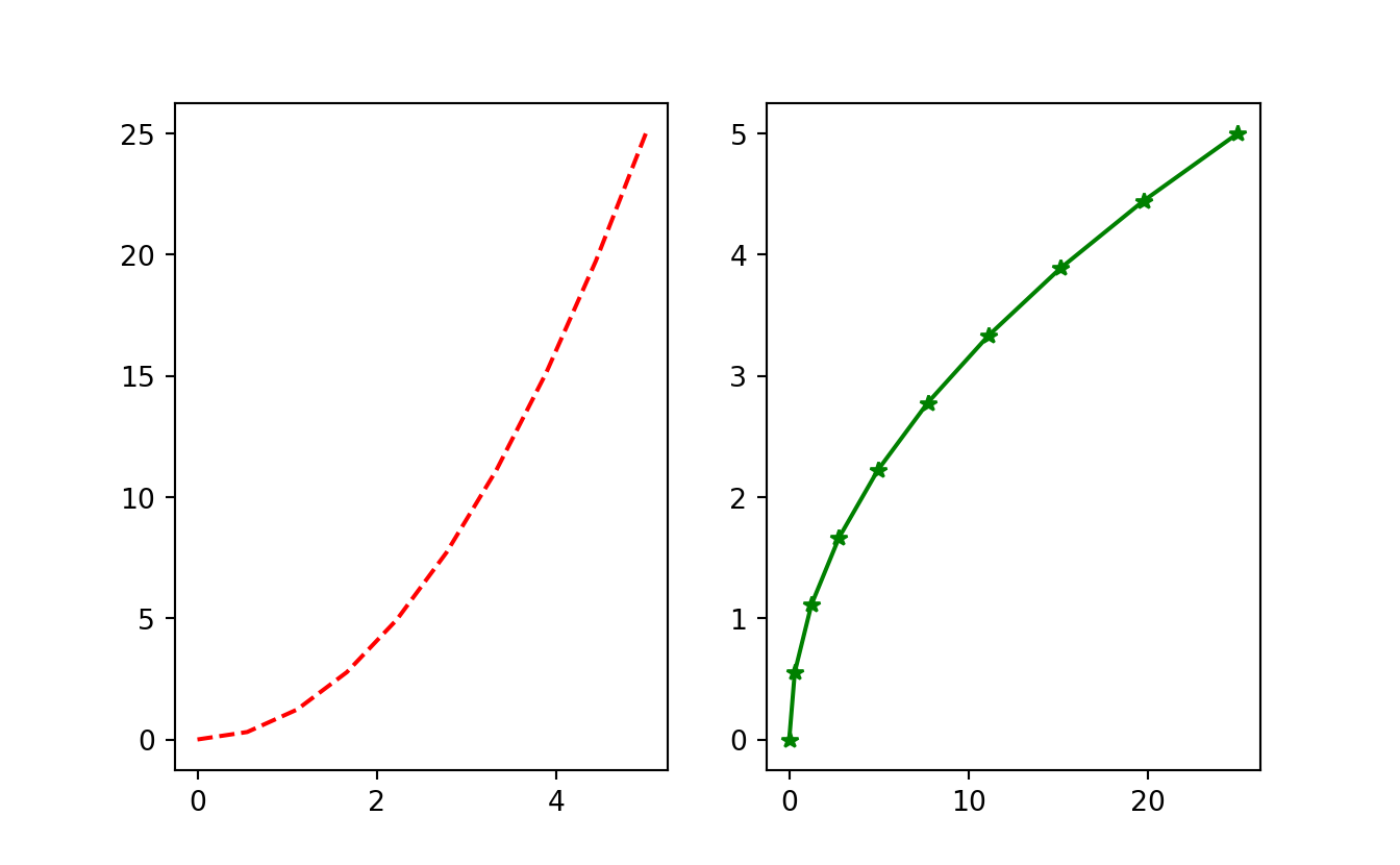
14.4.3 Multiple Axes In One Plot
- This is still considered a single plot, but with multiple axes
fig = plt.figure()
ax1 = fig.add_axes([0, 0, 1, 1])         # main axes
ax2 = fig.add_axes([0.2, 0.5, 0.4, 0.3]) # inset axes

ax1.plot(x,y,'r')
ax1.set_xlabel('x')
ax1.set_ylabel('y')

ax2.plot(y, x, 'g')
ax2.set_xlabel('y')
ax2.set_ylabel('x')
ax2.set_title('insert title')
plt.show()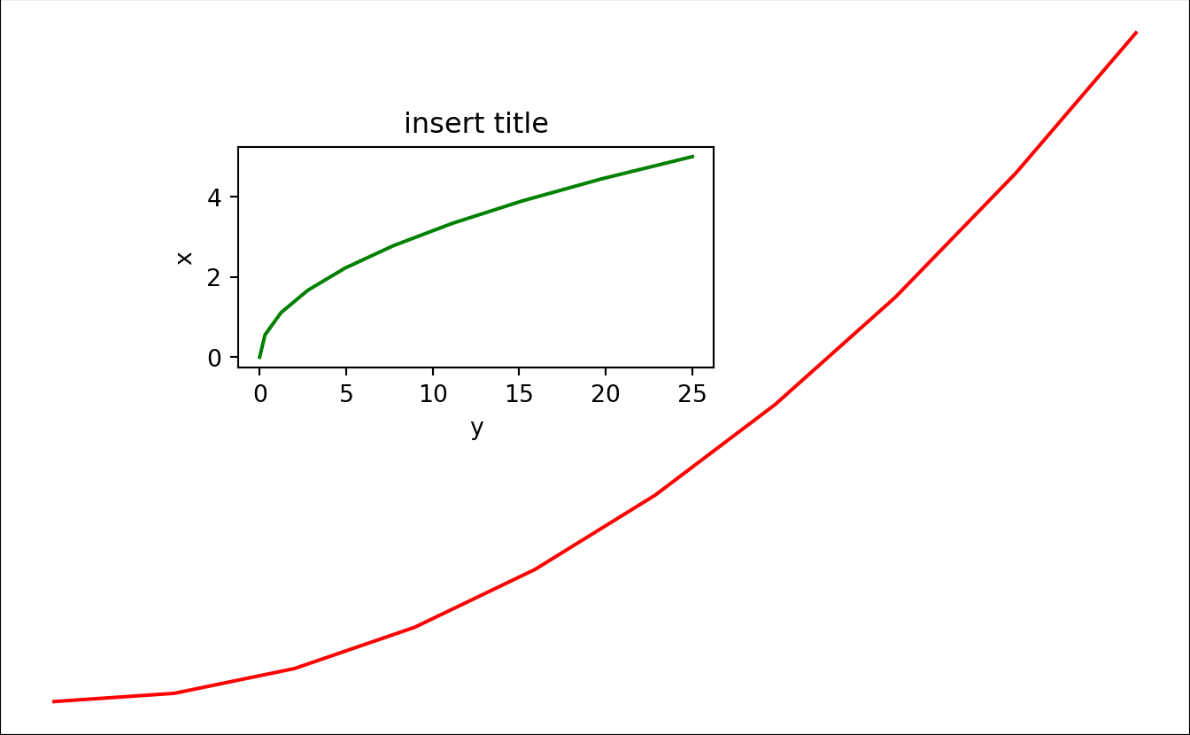
14.4.4 Multiple Subplots
- One figure can contain multiple subplots
- Each subplot has one axes
14.4.4.1 Simple Subplots - all same size
- subplots() function return axes object that is iterable.
Single Row Grid
Single row grid means axes is an 1-D array. Hence can use for to iterate through axes
fig, axes = plt.subplots( nrows=1,ncols=3 )
print (axes.shape)
for ax in axes:
ax.plot(x, y, 'r')
ax.set_xlabel('x')
ax.set_ylabel('y')
ax.set_title('title')
ax.text(0.2,0.5,'One')
plt.show()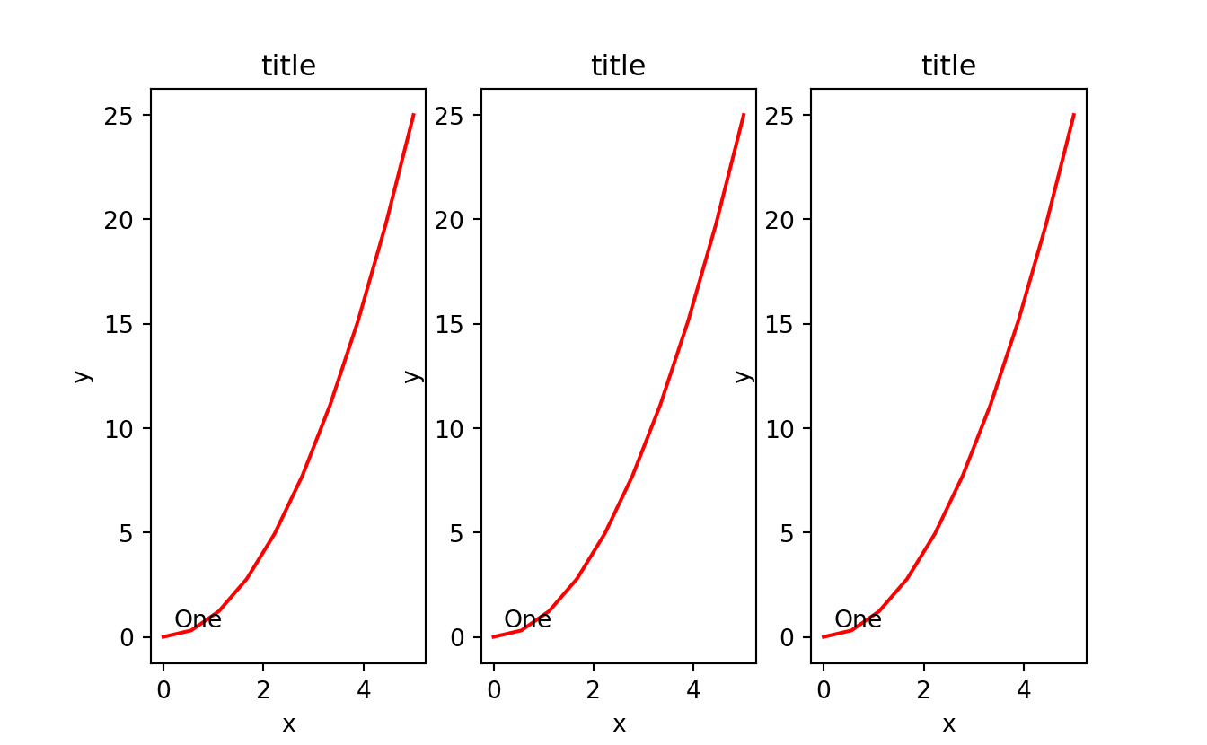
Multiple Row Grid
Multile row grid means axes is an 2-D array. Hence can use two levels of for loop to iterate through each row and column
fig, axes = plt.subplots(2, 3, sharex='col', sharey='row')
print (axes.shape)
for i in range(axes.shape[0]):
for j in range(axes.shape[1]):
axes[i, j].text(0.5, 0.5, str((i, j)),
fontsize=18, ha='center')
plt.show()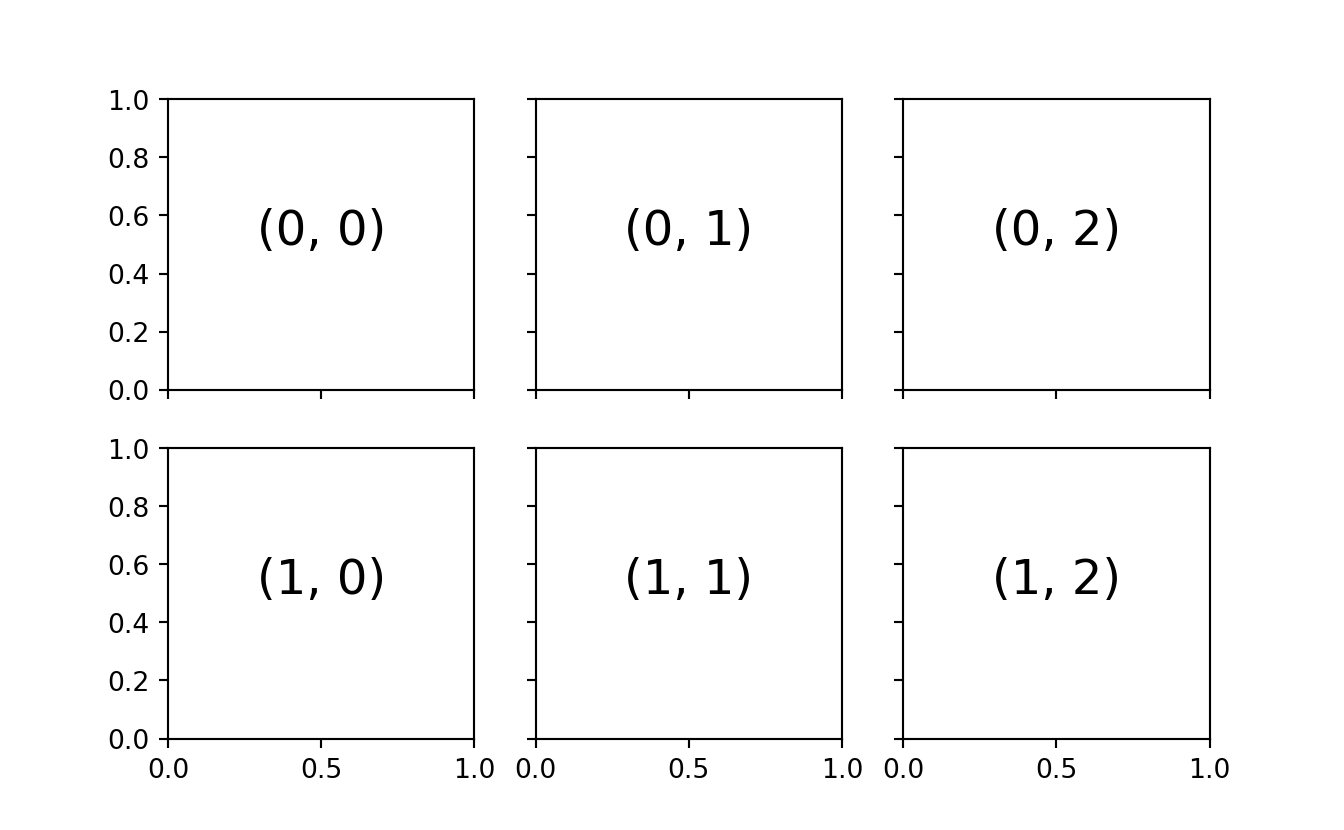
14.4.4.2 Complicated Subplots - different size
-
GridSpec specify grid size of the figure
- Manually specify each subplot and their relevant grid position and size
plt.figure(figsize=(5,5))
grid = plt.GridSpec(2, 3, hspace=0.4, wspace=0.4)
plt.subplot(grid[0, 0])  #row 0, col 0
plt.subplot(grid[0, 1:]) #row 0, col 1 to :
plt.subplot(grid[1, :2]) #row 1, col 0:2
plt.subplot(grid[1, 2]); #row 1, col 2
plt.show()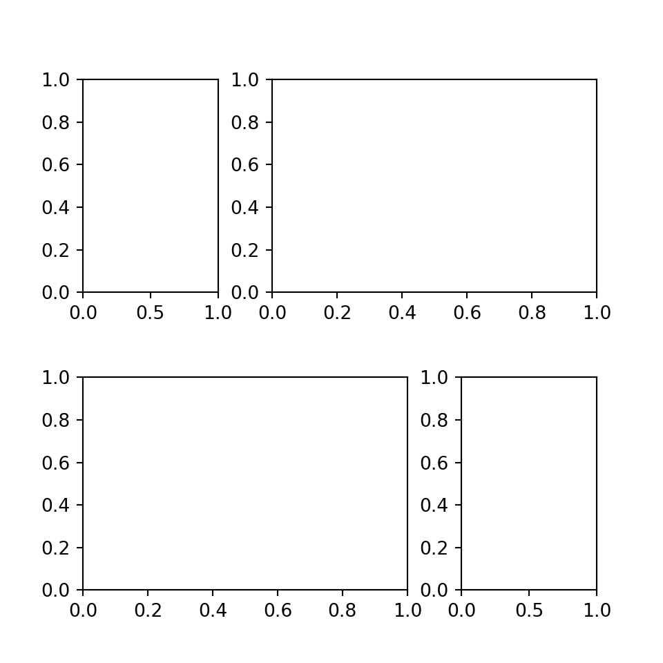
plt.figure(figsize=(5,5))
grid = plt.GridSpec(4, 4, hspace=0.8, wspace=0.4)
plt.subplot(grid[:3, 0])    # row 0:3, col 0
plt.subplot(grid[:3, 1: ])  # row 0:3, col 1:
plt.subplot(grid[3, 1: ]);  # row 3,   col 1:
plt.show()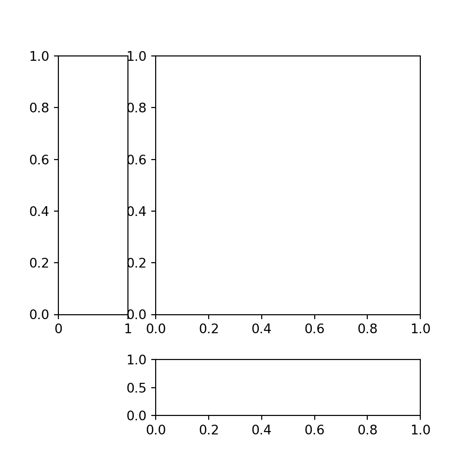
-1 means last row or column
plt.figure(figsize=(6,6))
grid = plt.GridSpec(4, 4, hspace=0.4, wspace=1.2)
plt.subplot(grid[:-1, 0 ])  # row 0 till last row (not including last row), col 0
plt.subplot(grid[:-1, 1:])  # row 0 till last row (not including last row), col 1 till end
plt.subplot(grid[-1, 1: ]); # row last row, col 1 till end
plt.show()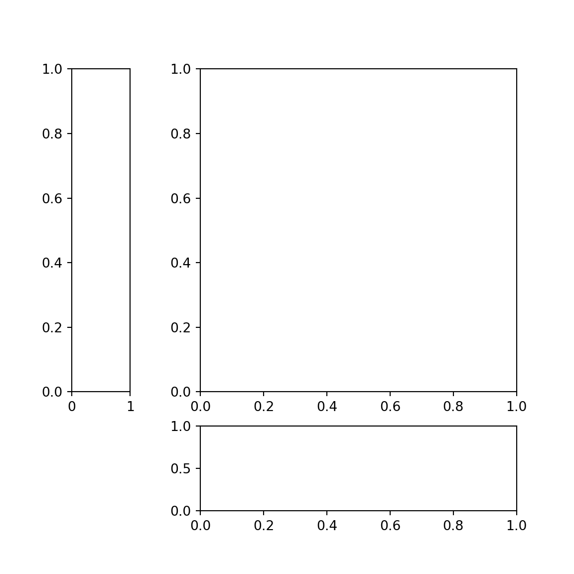
14.4.5 Figure Customization
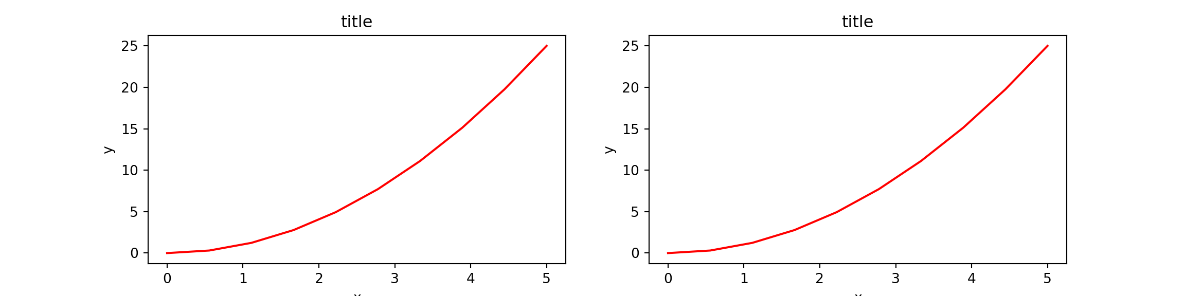
14.4.5.1 Avoid Overlap - Use tight_layout()
Sometimes when the figure size is too small, plots will overlap each other.
- tight_layout() will introduce extra white space in between the subplots to avoid overlap.
- The figure became wider.
fig, axes = plt.subplots( nrows=1,ncols=2)
for ax in axes:
    ax.plot(x, y, 'r')
    ax.set_xlabel('x')
    ax.set_ylabel('y')
    ax.set_title('title')
fig.tight_layout() # adjust the positions of axes so that there is no overlap
plt.show()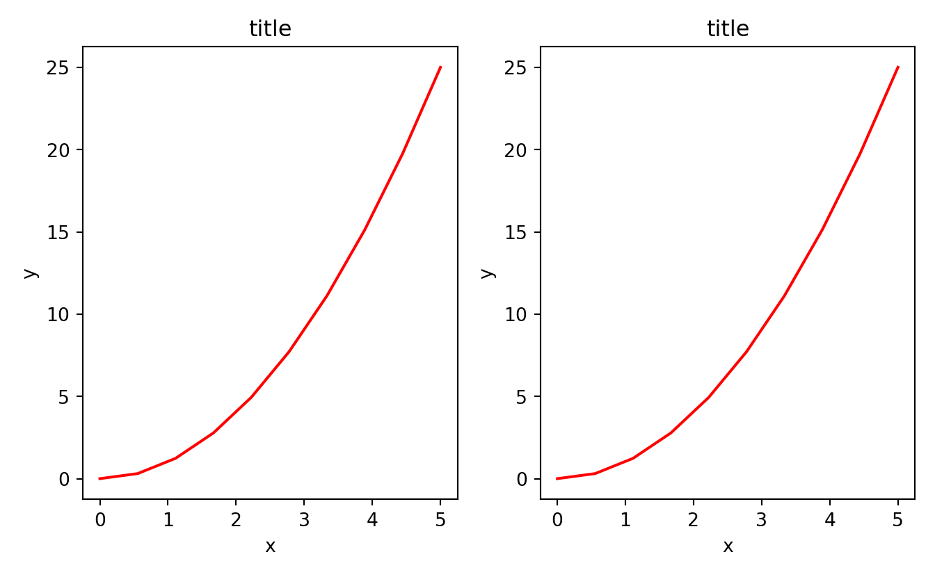

14.4.6 Axes Customization

14.4.6.2 Text Within Axes
fig, ax = plt.subplots(2, 3, sharex='col', sharey='row')
for i in range(2):
    for j in range(3):
        ax[i, j].text(0.5, 0.5, str((i, j)),
                      fontsize=18, ha='center')
plt.show()
plt.text(0.5, 0.5, 'one',fontsize=18, ha='center')
plt.show()
14.4.6.3 Share Y Axis Label
fig, ax = plt.subplots(2, 3, sharex='col', sharey='row') # removed inner label
plt.show()
14.4.6.4 Create Subplot Individually
Each call lto subplot() will create a new container for subsequent plot command
plt.subplot(2,4,1)
plt.text(0.5, 0.5, 'one',fontsize=18, ha='center')

plt.subplot(2,4,8)
plt.text(0.5, 0.5, 'eight',fontsize=18, ha='center')
plt.show()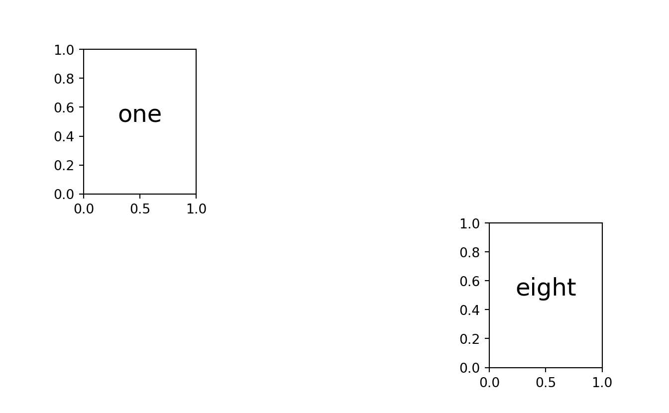
Iterate through subplots (ax) to populate them
fig, ax = plt.subplots(2, 3, sharex='col', sharey='row')
for i in range(2):
    for j in range(3):
        ax[i, j].text(0.5, 0.5, str((i, j)),
                      fontsize=18, ha='center')
plt.show()