Chapter 8 Example 1: A classification problem with Logistic Regression

8.1 Code in Python

I will combine here R and Python code just to show how easy is integrating R and Python. First thing we have to do is loading the package rTorch. We do that in a chunk:

library(rTorch)

Then, we proceed to copy the standard Python code but in their own Python chunks. This is a very nice example that I found in the web. It explains the classic challenge of classification.

When rTorch is loaded, a number of Python libraries are also loaded, which enable us the immediate use of numpy, torch and matplotlib.

# Logistic Regression
# https://m-alcu.github.io/blog/2018/02/10/logit-pytorch/
import numpy as np
import torch
import torch.nn.functional as F
from torch.autograd import Variable
import matplotlib.pyplot as plt

The next thing we do is setting a seed to make the example repeatable, in my machine and yours.

np.random.seed(2048)

Then we generate some random samples.

N = 100
D = 2
X = np.random.randn(N, D) * 2
ctr = int(N/2)
# center the first N/2 points at (-2,-2)
X[:ctr,:] = X[:ctr,:] - 2 * np.ones((ctr, D))
# center the last N/2 points at (2, 2)
X[ctr:,:] = X[ctr:,:] + 2 * np.ones((ctr, D))

# labels: first N/2 are 0, last N/2 are 1
# mark the first half with 0 and the sceond half with 1
T = np.array([0] * ctr + [1] * ctr).reshape(100, 1)

And plot the original data for reference.

# plot the data. color the dots using T
plt.scatter(X[:,0], X[:,1], c=T.reshape(N), s=100, alpha=0.5)
plt.xlabel('X(1)')
plt.ylabel('X(2)')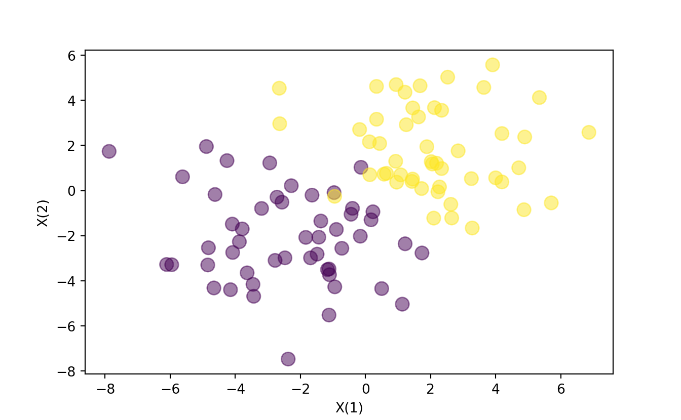

What follows is the definition of the model using a neural network and train the model. We set up the model:

class Model(torch.nn.Module):
    def __init__(self):
        super(Model, self).__init__()
        self.linear = torch.nn.Linear(2, 1) # 2 in and 1 out
        
    def forward(self, x):
        y_pred = torch.sigmoid(self.linear(x))
        return y_pred
    
# Our model    
model = Model()

criterion = torch.nn.BCELoss(reduction='mean')
optimizer = torch.optim.SGD(model.parameters(), lr=0.01)

Train the model:

x_data = Variable(torch.Tensor(X))
y_data = Variable(torch.Tensor(T))

# Training loop
for epoch in range(1000):
    # Forward pass: Compute predicted y by passing x to the model
    y_pred = model(x_data)
    
    # Compute and print loss
    loss = criterion(y_pred, y_data)
    # print(epoch, loss.data[0])
    
    # Zero gradients, perform a backward pass, and update the weights.
    optimizer.zero_grad()
    loss.backward()
    optimizer.step()
    
w = list(model.parameters())
w0 = w[0].data.numpy()
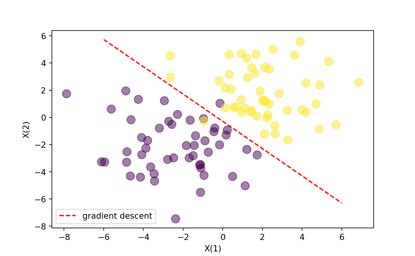
w1 = w[1].data.numpy()    

Finally, we plot the results, by tracing the line that separates two classes, 0 and 1, which are both colored in the plot.

print("Final gradient descend:", w)
# plot the data and separating line

#> Final gradient descend: [Parameter containing:
#> tensor([[1.0956, 1.1880]], requires_grad=True), Parameter containing:
#> tensor([0.2821], requires_grad=True)]

plt.scatter(X[:,0], X[:,1], c=T.reshape(N), s=100, alpha=0.5)
x_axis = np.linspace(-6, 6, 100)
y_axis = -(w1[0] + x_axis * w0[0][0]) / w0[0][1]
line_up, = plt.plot(x_axis, y_axis,'r--', label='gradient descent')
plt.legend(handles=[line_up])
plt.xlabel('X(1)')
plt.ylabel('X(2)')
plt.show()